Keras Tutorial
⚡ Smart Summary
Keras Tutorial introduces the high-level neural network API running on top of TensorFlow. Lessons cover what Keras is, architecture, models, layers, installation, training, evaluation, and comparison with TensorFlow for deep learning workflows.

What is Keras?
Keras is an Open Source Neural Network library written in Python that runs on top of Theano or Tensorflow. It is designed to be modular, fast and easy to use. It was developed by François Chollet, a Google engineer. Keras doesn’t handle low-level computation. Instead, it uses another library to do it, called the “Backend.
Keras is high-level API wrapper for the low-level API, capable of running on top of TensorFlow, CNTK, or Theano. Keras High-Level API handles the way we make models, defining layers, or set up multiple input-output models. In this level, Keras also compiles our model with loss and optimizer functions, training process with fit function. Keras in Python doesn’t handle Low-Level API such as making the computational graph, making tensors or other variables because it has been handled by the “backend” engine.
What is a Backend?
Backend is a term in Keras that performs all low-level computation such as tensor products, convolutions and many other things with the help of other libraries such as Tensorflow or Theano. So, the “backend engine” will perform the computation and development of the models. Tensorflow is the default “backend engine” but we can change it in the configuration.
Theano, Tensorflow, and CNTK Backend

Theano is an open source project that was developed by the MILA group at the University of Montreal, Quebec, Canada. It was the first widely used Framework. It is a Python library that helps in multi-dimensional arrays for mathematical operations using Numpy or Scipy. Theano can use GPUs for faster computation, it also can automatically build symbolic graphs for computing gradients. On its website, Theano claims that it can recognize numerically unstable expressions and compute them with more stable algorithms, this is very useful for our unstable expressions.

On the other hand, Tensorflow is the rising star in deep learning framework. Developed by Google’s Brain team it is the most popular deep learning tool. With a lot of features, and researchers contribute to help develop this framework for deep learning purposes.

Another backend engine for Keras is The Microsoft Cognitive Toolkit or CNTK. It is an open-source deep learning framework that was developed by Microsoft Team. It can run on multi GPUs or multi-machine for training deep learning model on a massive scale. In some cases, CNTK was reported faster than other frameworks such as Tensorflow or Theano. Next in this Keras CNN tutorial, we will compare the backends of Theano, TensorFlow and CNTK.
Comparing the Backends
We need to do a benchmark In order to know the comparison between these two backends. As you can see in Jeong-Yoon Lee’s benchmark, the performance of 3 different backends on different hardware is compared. And the result is Theano is slower than the other backend, it is reported 50 times slower, but the accuracy is close to each other.
Another benchmark test is performed by Jasmeet Bhatia. He reported that Theano is slower than Tensorflow for some test. But overall accuracy is nearly the same for every network that was tested.
So, between Theano, Tensorflow and CTK it’s obvious that TensorFlow is better than Theano. With TensorFlow, the computation time is much shorter and CNN is better than the others.
Next in this Keras Python tutorial, we will learn about the difference between Keras and TensorFlow (Keras vs Tensorflow).
Keras vs Tensorflow
| Parameters | Keras | Tensorflow |
|---|---|---|
| Type | High-Level API Wrapper | Low-Level API |
| Complexity | Easy to use if you Python language | You need to learn the syntax of using some of Tensorflow function |
| Purpose | Rapid deployment for making model with standard layers | Allows you to make an arbitrary computational graph or model layers |
| Tools | Uses other API debug tool such as TFDBG | You can use Tensorboard visualization tools |
| Community | Large active communities | Large active communities and widely shared resources |
Advantages of Keras
Fast Deployment and Easy to understand
Keras is very quick to make a network model. If you want to make a simple network model with a few lines, Python Keras can help you with that. Look at the Keras example below:
from keras.models import Sequential
from keras.layers import Dense, Activation

model = Sequential()
model.add(Dense(64, activation='relu', input_dim=50)) #input shape of 50
model.add(Dense(28, activation='relu')) #input shape of 50
model.add(Dense(10, activation='softmax'))
Because of friendly the API, we can easily understand the process. Writing the code with a simple function and no need to set multiple parameters.
Large Community Support
There are lots of AI communities that use Keras for their Deep Learning framework. Many of them publish their codes as well tutorials to the general public.
Have multiple Backends
You can choose Tensorflow, CNTK, and Theano as your backend with Keras. You can choose a different backend for different projects depending on your needs. Each backend has its own unique advantage.
Cross-Platform and Easy Model Deployment
With a variety of supported devices and platforms, you can deploy Keras on any device like
- iOS with CoreML
- Android with Tensorflow Android,
- Web browser with .js support
- Cloud engine
- Raspberry Pi
Multi GPUs Support
You can train Keras on a single GPU or use multiple GPUs at once. Because Keras has a built-in support for data parallelism so it can process large volumes of data and speed up the time needed to train it.
Disadvantages of Keras
Cannot handle low-level API
Keras only handles high-level API which runs on top other framework or backend engine such as Tensorflow, Theano, or CNTK. So it’s not very useful if you want to make your own abstract layer for your research purposes because Keras already have pre-configured layers.
Installing Keras
In this section, we will look into various methods available to install Keras
Direct install or Virtual Environment
Which one is better? Direct install to the current python or use a virtual environment? I suggest using a virtual environment if you have many projects. Want to know why? This is because different projects may use a different version of a keras library.
For example, I have a project that needs Python 3.5 using OpenCV 3.3 with older Keras-Theano backend but in the other project I have to use Keras with the latest version and a Tensorflow as it backend with Python 3.6.6 support
We don’t want the Keras library to conflict at each other right? So we use a Virtual Environment to localize the project with a specific type of library or we can use another platform such as Cloud Service to do our computation for us like Amazon Web Service.
Installing Keras on Amazon Web Service (AWS)
Amazon Web Service is a platform that offers Cloud Computing service and products for researchers or any other purposes. AWS rent their hardware, networking, Database, etc. so that we can use it directly from the internet. One of the popular AWS service for deep learning purpose is the Amazon Machine Image Deep Learning Service or DL
For detailed instructions on how to use AWS, refer this tutorial
Note on the AMI: You will have the following AMI available
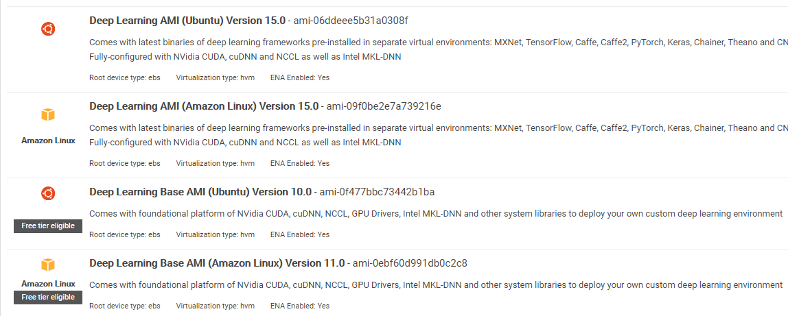
AWS Deep Learning AMI is a virtual environment in AWS EC2 Service that helps researchers or practitioners to work with Deep Learning. DLAMI offers from small CPUs engine up to high-powered multi GPUs engines with preconfigured CUDA, cuDNN, and comes with a variety of deep learning frameworks.
If you want to use it instantly, you should choose Deep Learning AMI because it comes preinstalled with popular deep learning frameworks.
But if you want to try a custom deep learning framework for research, you should install the Deep Learning Base AMI because it comes with fundamental libraries such as CUDA, cuDNN, GPUs drivers, and other needed libraries to run with your deep learning environment.
How to Install Keras on Amazon SageMaker
Amazon SageMaker is a deep learning platform to help you with training and deploying deep learning network with the best algorithm.
As a beginner, this is by far the easiest method to use Keras. Below is a process on how to install Keras on Amazon SageMaker:
Step 1) Open Amazon SageMaker
In the first step, Open the Amazon Sagemaker console and click on Create notebook instance.

Step 2) Enter the details
- Enter your notebook name.
- Create an IAM role. It will create an AMI role Amazon IAM role in the format of AmazonSageMaker-Executionrole-YYYYMMDD|HHmmSS.
- Finally, choose Create notebook instance. After a few moments, Amazon Sagemaker launches a notebook instance.

Note: If you want to access resources from your VPC, set the direct internet access as enabled. Otherwise, this notebook instance will not have an internet access, so it is impossible to train or host models
Step 3) Launch the instance
Click on Open to launch the instance

Step 4) Start coding
In Jupyter, Click on New> conda_tensorflow_p36 and you are ready to code

Install Keras in Linux
To enable Keras with Tensorflow as its backend engine, we need to install Tensorflow first. Run this command to install tensorflow with CPU (no GPU)
pip install --upgrade tensorflow
if you want to enable the GPU support for tensorflow you can use this command
pip install --upgrade tensorflow-gpu

let’s check in Python to see if our installation is successful by typing
user@user:~$ python
Python 3.6.4 (default, Mar 20 2018, 11:10:20)
[GCC 5.4.0 20160609] on linux
Type "help", "copyright", "credits" or "license" for more information.
>>> import tensorflow
>>>
if there is no error message, the installation process is successful
Install Keras
After we install Tensorflow, let’s start installing keras. Type this command in the terminal
pip install keras
it will begin installing Keras and also all of its dependencies.You should see something like this :

Now we have Keras Installed in our system!
Verifying
Before we start using Keras, we should check if our Keras use Tensorflow as it backend by open the configuration file:
gedit ~/.keras/keras.json
you should see something like this
{
    "floatx": "float32",
    "epsilon": 1e-07,
    "backend": "tensorflow",
    "image_data_format": "channels_last"
}
as you can see, the “backend” use tensorflow. It means that keras are using Tensorflow as it backend as we expected
and now run it on the terminal by typing
user@user:~$ python3
Python 3.6.4 (default, Mar 20 2018, 11:10:20)
[GCC 5.4.0 20160609] on linux
Type "help", "copyright", "credits" or "license" for more information.
>>> import keras
Using TensorFlow backend.
>>>
How to Install Keras on Windows
Before we install Tensorflow and Keras, we should install Python, pip, and virtualenv. If you already installed these libraries, you should continue to the next step, otherwise do this:
Install Python 3 by downloading from this link
Install pip by running this
Install virtualenv with this command
pip3 install –U pip virtualenv
Install Microsoft Visual C++ 2015 Redistributable Update 3
- Go to the Visual Studio download site https://www.microsoft.com/en-us/download/details.aspx?id=53587
- Select Redistributables and Build Tools
- Download and install the Microsoft Visual C++ 2015 Redistributable Update 3
Then run this script
pip3 install virtualenv
Setup Virtual Environment
This is used to isolate the working system with the main system.
virtualenv –-system-site-packages –p python3 ./venv
Activate the environment
.\venv\Scripts\activate
After preparing the environment, Tensorflow and Keras installation remains same as Linux. Next in this Deep learning with Keras tutorial, we will learn about Keras fundamentals for Deep learning.
Keras Fundamentals for Deep Learning
The main structure in Keras is the Model which defines the complete graph of a network. You can add more layers to an existing model to build a custom model that you need for your project.
Here’s how to make a Sequential Model and a few commonly used layers in deep learning
1. Sequential Model
from keras.models import Sequential
from keras.layers import Dense, Activation,Conv2D,MaxPooling2D,Flatten,Dropout

model = Sequential()
2. Convolutional Layer
This is a Keras Python example of convolutional layer as the input layer with the input shape of 320x320x3, with 48 filters of size 3×3 and use ReLU as an activation function.
input_shape=(320,320,3) #this is the input shape of an image 320x320x3
model.add(Conv2D(48, (3, 3), activation='relu', input_shape= input_shape))
another type is
model.add(Conv2D(48, (3, 3), activation='relu'))
3. MaxPooling Layer
To downsample the input representation, use MaxPool2d and specify the kernel size
model.add(MaxPooling2D(pool_size=(2, 2)))
4. Dense Layer
adding a Fully Connected Layer with just specifying the output Size
model.add(Dense(256, activation='relu'))
5. Dropout Layer
Adding dropout layer with 50% probability
model.add(Dropout(0.5))
Compiling, Training, and Evaluate
After we define our model, let’s start to train them. It is required to compile the network first with the loss function and optimizer function. This will allow the network to change weights and minimized the loss.
model.compile(loss='mean_squared_error', optimizer='adam')
Now to start training, use fit to fed the training and validation data to the model. This will allow you to train the network in batches and set the epochs.
model.fit(X_train, X_train, batch_size=32, epochs=10, validation_data=(x_val, y_val))
Our final step is to evaluate the model with the test data.
score = model.evaluate(x_test, y_test, batch_size=32)
Lets try using simple linear regression
import keras
from keras.models import Sequential
from keras.layers import Dense, Activation
import numpy as np
import matplotlib.pyplot as plt

x = data = np.linspace(1,2,200)
y = x*4 + np.random.randn(*x.shape) * 0.3


model = Sequential()
model.add(Dense(1, input_dim=1, activation='linear'))

model.compile(optimizer='sgd', loss='mse', metrics=['mse'])

weights = model.layers[0].get_weights()
w_init = weights[0][0][0]
b_init = weights[1][0]
print('Linear regression model is initialized with weights w: %.2f, b: %.2f' % (w_init, b_init))


model.fit(x,y, batch_size=1, epochs=30, shuffle=False)

weights = model.layers[0].get_weights()
w_final = weights[0][0][0]
b_final = weights[1][0]
print('Linear regression model is trained to have weight w: %.2f, b: %.2f' % (w_final, b_final))

predict = model.predict(data)

plt.plot(data, predict, 'b', data , y, 'k.')
plt.show()
After training the data, the output should look like this
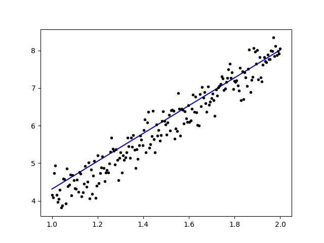
with the initial weight
Linear regression model is initialized with weights w: 0.37, b: 0.00
and final weight
Linear regression model is trained to have weight w: 3.70, b: 0.61
Fine-Tune Pre-Trained Models in Keras and How to Use Them
Why we use Fine Tune Models and when we use it
Fine-tuning is a task to tweak a pre-trained model such that the parameters would adapt to the new model. When we want to train from scratch on a new model, we need a large amount of data, so that the network can find all parameters. But in this case, we will use a pre-trained model so the parameters are already learned and have a weight.
For example, if we want to train our own Keras model to solve a classification problem but we only have a small amount of data, then we can solve this by using a Transfer Learning + Fine-Tuning method.
Using a pre-trained network & weights we don’t need to train the whole network. We just need to train the last layer that is used to solve our task as we call it Fine-Tuning method.
Network Model Preparation
For the pre-trained model, we can load a variety of models that Keras already has in its library such as:
- VGG16
- InceptionV3
- ResNet
- MobileNet
- Xception
- InceptionResNetV2
But in this process, we will use VGG16 network model and the imageNet as our weight for the model. We will fine-tune a network to classify 8 different types of classes using Images from Kaggle Natural Images Dataset
VGG16 model architecture

Uploading Our Data to AWS S3 Bucket
For our training process, we will use a picture of natural images from 8 different classes such as airplanes, car, cat, dog, flower, fruit, motorbike, and person. First, we need to upload our data to Amazon S3 Bucket.
Amazon S3 Bucket
Step 1) After login to your S3 account, let’s create a bucket by clocking Create Bucket

Step 2) Now choose a Bucket Name and your Region according to your account. Make sure that the bucket name is available. After that click Create.

Step 3) As you can see, your Bucket is ready to use. But as you can see, the Access is Not public, it is good for you if you want to keep it private for yourself. You can change this bucket for Public Access in the Bucket Properties

Step 4) Now you start uploading your training data to your Bucket. Here I will upload the tar.gz file which consist of pictures for training and testing process.

Step 5) Now click on your file and copy the Link so that we can download it.

Data Preparation
We need to generate our training data using the Keras ImageDataGenerator.
First you must download using wget with the link to your file from S3 Bucket.
!wget https://s3.us-east-2.amazonaws.com/naturalimages02/images.tar.gz
!tar -xzf images.tar.gz
After you download the data let’s start the Training Process.
from keras.preprocessing.image import ImageDataGenerator
import numpy as np
import matplotlib.pyplot as plt

train_path = 'images/train/'
test_path = 'images/test/'
batch_size = 16
image_size = 224
num_class = 8


train_datagen = ImageDataGenerator(validation_split=0.3,
                                   shear_range=0.2,
                                   zoom_range=0.2,
                                   horizontal_flip=True)

train_generator = train_datagen.flow_from_directory(
                        directory=train_path,
                        target_size=(image_size,image_size),
                        batch_size=batch_size,
                        class_mode='categorical',
                        color_mode='rgb',
                        shuffle=True)
The ImageDataGenerator will make an X_training data from a directory. The sub-directory in that directory will be used as a class for each object. The image will be loaded with the RGB color mode, with the categorical class mode for the Y_training data, with a batch size of 16. Finally, shuffle the data.
Let’s see our images randomly by plotting them with matplotlib
x_batch, y_batch = train_generator.next()

fig=plt.figure()
columns = 4
rows = 4
for i in range(1, columns*rows):
    num = np.random.randint(batch_size)
    image = x_batch[num].astype(np.int)
    fig.add_subplot(rows, columns, i)
    plt.imshow(image)
plt.show()

After that let’s create our network model from VGG16 with imageNet pre-trained weight. We will freeze these layers so that the layers are not trainable to help us reduce the computation time.
Creating our Model from VGG16
import keras
from keras.models import Model, load_model
from keras.layers import Activation, Dropout, Flatten, Dense
from keras.preprocessing.image import ImageDataGenerator
from keras.applications.vgg16 import VGG16


#Load the VGG model
base_model = VGG16(weights='imagenet', include_top=False, input_shape=(image_size, image_size, 3))

print(base_model.summary())

    # Freeze the layers
for layer in base_model.layers:
    layer.trainable = False

# # Create the model
model = keras.models.Sequential()

# # Add the vgg convolutional base model
model.add(base_model)

# # Add new layers
model.add(Flatten())
model.add(Dense(1024, activation='relu'))
model.add(Dense(1024, activation='relu'))
model.add(Dense(num_class, activation='softmax'))

# # Show a summary of the model. Check the number of trainable parameters
print(model.summary())
As you can see below, the summary of our network model. From an input from VGG16 Layers, then we add 2 Fully Connected Layer which will extract 1024 features and an output layer that will compute the 8 classes with the softmax activation.
Layer (type)                 Output Shape              Param #
=================================================================
vgg16 (Model)                (None, 7, 7, 512)         14714688
_________________________________________________________________
flatten_1 (Flatten)          (None, 25088)             0
_________________________________________________________________
dense_1 (Dense)              (None, 1024)              25691136
_________________________________________________________________
dense_2 (Dense)              (None, 1024)              1049600
_________________________________________________________________
dense_3 (Dense)              (None, 8)                 8200
=================================================================
Total params: 41,463,624
Trainable params: 26,748,936
Non-trainable params: 14,714,688
Training
# # Compile the model
from keras.optimizers import SGD

model.compile(loss='categorical_crossentropy',
          optimizer=SGD(lr=1e-3),
          metrics=['accuracy'])

# # Start the training process
# model.fit(x_train, y_train, validation_split=0.30, batch_size=32, epochs=50, verbose=2)

# # #save the model
# model.save('catdog.h5')

history = model.fit_generator(
        train_generator,
        steps_per_epoch=train_generator.n/batch_size,
        epochs=10)

model.save('fine_tune.h5')

# summarize history for accuracy
import matplotlib.pyplot as plt

plt.plot(history.history['loss'])
plt.title('loss')
plt.ylabel('loss')
plt.xlabel('epoch')
plt.legend(['loss'], loc='upper left')
plt.show()
Results
Epoch 1/10
432/431 [==============================] - 53s 123ms/step - loss: 0.5524 - acc: 0.9474
Epoch 2/10
432/431 [==============================] - 52s 119ms/step - loss: 0.1571 - acc: 0.9831
Epoch 3/10
432/431 [==============================] - 51s 119ms/step - loss: 0.1087 - acc: 0.9871
Epoch 4/10
432/431 [==============================] - 51s 119ms/step - loss: 0.0624 - acc: 0.9926
Epoch 5/10
432/431 [==============================] - 51s 119ms/step - loss: 0.0591 - acc: 0.9938
Epoch 6/10
432/431 [==============================] - 51s 119ms/step - loss: 0.0498 - acc: 0.9936
Epoch 7/10
432/431 [==============================] - 51s 119ms/step - loss: 0.0403 - acc: 0.9958
Epoch 8/10
432/431 [==============================] - 51s 119ms/step - loss: 0.0248 - acc: 0.9959
Epoch 9/10
432/431 [==============================] - 51s 119ms/step - loss: 0.0466 - acc: 0.9942
Epoch 10/10
432/431 [==============================] - 52s 120ms/step - loss: 0.0338 - acc: 0.9947

As you can see, our losses are dropped significantly and the accuracy is almost 100%. For testing our model, we randomly picked images over the internet and put it on the test folder with a different class to test
Testing Our Model
model = load_model('fine_tune.h5')

test_datagen = ImageDataGenerator()
train_generator = train_datagen.flow_from_directory(
                        directory=train_path,
                        target_size=(image_size,image_size),
                        batch_size=batch_size,
                        class_mode='categorical',
                        color_mode='rgb',
                        shuffle=True)

test_generator = test_datagen.flow_from_directory(
                        directory=test_path,
                        target_size=(image_size, image_size),
                        color_mode='rgb',
                        shuffle=False,
                        class_mode='categorical',
                        batch_size=1)

filenames = test_generator.filenames
nb_samples = len(filenames)

fig=plt.figure()
columns = 4
rows = 4
for i in range(1, columns*rows -1):
    x_batch, y_batch = test_generator.next()

    name = model.predict(x_batch)
    name = np.argmax(name, axis=-1)
    true_name = y_batch
    true_name = np.argmax(true_name, axis=-1)

    label_map = (test_generator.class_indices)
    label_map = dict((v,k) for k,v in label_map.items()) #flip k,v
    predictions = [label_map[k] for k in name]
    true_value = [label_map[k] for k in true_name]

    image = x_batch[0].astype(np.int)
    fig.add_subplot(rows, columns, i)
    plt.title(str(predictions[0]) + ':' + str(true_value[0]))
    plt.imshow(image)
plt.show()
And our test is as given below! Only 1 image is predicted wrong from a test of 14 images!

Face Recognition Neural Network with Keras
Why we need Recognition
We need Recognition to make it easier for us to recognize or identify a person’s face, objects type, estimated age of a person from his face, or even know the facial expressions of that person.

Maybe you realize every time you try to mark your friend’s face in a photo, the feature in Facebook has done it for you, that is marking your friend’s face without you needing to mark it first. This is Face Recognition applied by Facebook to make it easier for us to tag friends.
So how does it work? Every time we mark the face of our friend, Facebook’s AI will learn it and will try to predict it until it gets the right result. The same system we will use to make our own Face Recognition. Let’s start making our own Face Recognition using Deep Learning
Network Model
We will use a VGG16 Network Model but with VGGFace weight.
VGG16 model architecture

What is VGGFace? it is Keras implementation of Deep Face Recognition introduced by Parkhi, Omkar M. et al. “Deep Face Recognition.” BMVC (2015). The framework uses VGG16 as the network architecture.
You can download the VGGFace from github
from keras.applications.vgg16 import VGG16
from keras_vggface.vggface import VGGFace

face_model = VGGFace(model='vgg16',
                weights='vggface',
                input_shape=(224,224,3))
face_model.summary()
As you can see the network summary
_________________________________________________________________
Layer (type)                 Output Shape              Param #
=================================================================
input_1 (InputLayer)         (None, 224, 224, 3)       0
_________________________________________________________________
conv1_1 (Conv2D)             (None, 224, 224, 64)      1792
_________________________________________________________________
conv1_2 (Conv2D)             (None, 224, 224, 64)      36928
_________________________________________________________________
pool1 (MaxPooling2D)         (None, 112, 112, 64)      0
_________________________________________________________________
conv2_1 (Conv2D)             (None, 112, 112, 128)     73856
_________________________________________________________________
conv2_2 (Conv2D)             (None, 112, 112, 128)     147584
_________________________________________________________________
pool2 (MaxPooling2D)         (None, 56, 56, 128)       0
_________________________________________________________________
conv3_1 (Conv2D)             (None, 56, 56, 256)       295168
_________________________________________________________________
conv3_2 (Conv2D)             (None, 56, 56, 256)       590080
_________________________________________________________________
conv3_3 (Conv2D)             (None, 56, 56, 256)       590080
_________________________________________________________________
pool3 (MaxPooling2D)         (None, 28, 28, 256)       0
_________________________________________________________________
conv4_1 (Conv2D)             (None, 28, 28, 512)       1180160
_________________________________________________________________
conv4_2 (Conv2D)             (None, 28, 28, 512)       2359808
_________________________________________________________________
conv4_3 (Conv2D)             (None, 28, 28, 512)       2359808
_________________________________________________________________
pool4 (MaxPooling2D)         (None, 14, 14, 512)       0
_________________________________________________________________
conv5_1 (Conv2D)             (None, 14, 14, 512)       2359808
_________________________________________________________________
conv5_2 (Conv2D)             (None, 14, 14, 512)       2359808
_________________________________________________________________
conv5_3 (Conv2D)             (None, 14, 14, 512)       2359808
_________________________________________________________________
pool5 (MaxPooling2D)         (None, 7, 7, 512)         0
_________________________________________________________________
flatten (Flatten)            (None, 25088)             0
_________________________________________________________________
fc6 (Dense)                  (None, 4096)              102764544
_________________________________________________________________
fc6/relu (Activation)        (None, 4096)              0
_________________________________________________________________
fc7 (Dense)                  (None, 4096)              16781312
_________________________________________________________________
fc7/relu (Activation)        (None, 4096)              0
_________________________________________________________________
fc8 (Dense)                  (None, 2622)              10742334
_________________________________________________________________
fc8/softmax (Activation)     (None, 2622)              0
=================================================================
Total params: 145,002,878
Trainable params: 145,002,878
Non-trainable params: 0
_________________________________________________________________
Traceback (most recent call last):
we will do a Transfer Learning + Fine Tuning to make the training quicker with small datasets. First, we will freeze the base layers so that the layers are not trainable.
for layer in face_model.layers:
    layer.trainable = False
then we add our own layer to recognize our test faces. We will add 2 fully connected layer and an output layer with 5 people to detect.
from keras.models import Model, Sequential
from keras.layers import Input, Convolution2D, ZeroPadding2D, MaxPooling2D, Flatten, Dense, Dropout, Activation

person_count = 5

last_layer = face_model.get_layer('pool5').output

x = Flatten(name='flatten')(last_layer)
x = Dense(1024, activation='relu', name='fc6')(x)
x = Dense(1024, activation='relu', name='fc7')(x)
out = Dense(person_count, activation='softmax', name='fc8')(x)

custom_face = Model(face_model.input, out)
Let’s see our network summary
Layer (type)                 Output Shape              Param #
=================================================================
input_1 (InputLayer)         (None, 224, 224, 3)       0
_________________________________________________________________
conv1_1 (Conv2D)             (None, 224, 224, 64)      1792
_________________________________________________________________
conv1_2 (Conv2D)             (None, 224, 224, 64)      36928
_________________________________________________________________
pool1 (MaxPooling2D)         (None, 112, 112, 64)      0
_________________________________________________________________
conv2_1 (Conv2D)             (None, 112, 112, 128)     73856
_________________________________________________________________
conv2_2 (Conv2D)             (None, 112, 112, 128)     147584
_________________________________________________________________
pool2 (MaxPooling2D)         (None, 56, 56, 128)       0
_________________________________________________________________
conv3_1 (Conv2D)             (None, 56, 56, 256)       295168
_________________________________________________________________
conv3_2 (Conv2D)             (None, 56, 56, 256)       590080
_________________________________________________________________
conv3_3 (Conv2D)             (None, 56, 56, 256)       590080
_________________________________________________________________
pool3 (MaxPooling2D)         (None, 28, 28, 256)       0
_________________________________________________________________
conv4_1 (Conv2D)             (None, 28, 28, 512)       1180160
_________________________________________________________________
conv4_2 (Conv2D)             (None, 28, 28, 512)       2359808
_________________________________________________________________
conv4_3 (Conv2D)             (None, 28, 28, 512)       2359808
_________________________________________________________________
pool4 (MaxPooling2D)         (None, 14, 14, 512)       0
_________________________________________________________________
conv5_1 (Conv2D)             (None, 14, 14, 512)       2359808
_________________________________________________________________
conv5_2 (Conv2D)             (None, 14, 14, 512)       2359808
_________________________________________________________________
conv5_3 (Conv2D)             (None, 14, 14, 512)       2359808
_________________________________________________________________
pool5 (MaxPooling2D)         (None, 7, 7, 512)         0
_________________________________________________________________
flatten (Flatten)            (None, 25088)             0
_________________________________________________________________
fc6 (Dense)                  (None, 1024)              25691136
_________________________________________________________________
fc7 (Dense)                  (None, 1024)              1049600
_________________________________________________________________
fc8 (Dense)                  (None, 5)                 5125
=================================================================
Total params: 41,460,549
Trainable params: 26,745,861
Non-trainable params: 14,714,688
As you can see above, after the pool5 layer, it will be flattened into a single feature vector that will be used by the dense layer for the final recognition.
Preparing our Faces
Now let’s prepare our faces. I made a directory consist of 5 famous people
- Jack Ma
- Jason Statham
- Johnny Depp
- Robert Downey Jr
- Rowan Atkinson
Each folder contains 10 pictures, for each training and evaluation process. It is a very small amount of data but that is the challenge, right?
We will use the help of Keras tool to help us prepare the data. This function will iterate in the dataset folder and then prepare it so it can be used in the training.
from keras.preprocessing.image import ImageDataGenerator
batch_size = 5
train_path = 'data/'
eval_path = 'eval/'

train_datagen = ImageDataGenerator(rescale=1./255,
                                   shear_range=0.2,
                                   zoom_range=0.2,
                                   horizontal_flip=True)

valid_datagen = ImageDataGenerator(rescale=1./255,
                                   shear_range=0.2,
                                   zoom_range=0.2,
                                   horizontal_flip=True)

train_generator = train_datagen.flow_from_directory(
                        train_path,
                        target_size=(image_size,image_size),
                        batch_size=batch_size,
                        class_mode='sparse',
                        color_mode='rgb')

valid_generator = valid_datagen.flow_from_directory(
    directory=eval_path,
    target_size=(224, 224),
    color_mode='rgb',
    batch_size=batch_size,
    class_mode='sparse',
    shuffle=True,
)
Training Our Model
Let’s begin our training process by compiling our network with loss function and optimizer. Here, we use sparse_categorical_crossentropy as our loss function, with the help of SGD as our learning optimizer.
from keras.optimizers import SGD

custom_face.compile(loss='sparse_categorical_crossentropy',
                         optimizer=SGD(lr=1e-4, momentum=0.9),
                         metrics=['accuracy'])

history = custom_face.fit_generator(
        train_generator,
        validation_data=valid_generator,
        steps_per_epoch=49/batch_size,
        validation_steps=valid_generator.n,
        epochs=50)

custom_face.evaluate_generator(generator=valid_generator)

custom_face.save('vgg_face.h5')
Epoch 25/50
10/9 [==============================] - 60s 6s/step - loss: 1.4882 - acc: 0.8998 - val_loss: 1.5659 - val_acc: 0.5851
Epoch 26/50
10/9 [==============================] - 59s 6s/step - loss: 1.4882 - acc: 0.8998 - val_loss: 1.5638 - val_acc: 0.5809
Epoch 27/50
10/9 [==============================] - 60s 6s/step - loss: 1.4779 - acc: 0.8597 - val_loss: 1.5613 - val_acc: 0.5477
Epoch 28/50
10/9 [==============================] - 60s 6s/step - loss: 1.4755 - acc: 0.9199 - val_loss: 1.5576 - val_acc: 0.5809
Epoch 29/50
10/9 [==============================] - 60s 6s/step - loss: 1.4794 - acc: 0.9153 - val_loss: 1.5531 - val_acc: 0.5892
Epoch 30/50
10/9 [==============================] - 60s 6s/step - loss: 1.4714 - acc: 0.8953 - val_loss: 1.5510 - val_acc: 0.6017
Epoch 31/50
10/9 [==============================] - 60s 6s/step - loss: 1.4552 - acc: 0.9199 - val_loss: 1.5509 - val_acc: 0.5809
Epoch 32/50
10/9 [==============================] - 60s 6s/step - loss: 1.4504 - acc: 0.9199 - val_loss: 1.5492 - val_acc: 0.5975
Epoch 33/50
10/9 [==============================] - 60s 6s/step - loss: 1.4497 - acc: 0.8998 - val_loss: 1.5490 - val_acc: 0.5851
Epoch 34/50
10/9 [==============================] - 60s 6s/step - loss: 1.4453 - acc: 0.9399 - val_loss: 1.5529 - val_acc: 0.5643
Epoch 35/50
10/9 [==============================] - 60s 6s/step - loss: 1.4399 - acc: 0.9599 - val_loss: 1.5451 - val_acc: 0.5768
Epoch 36/50
10/9 [==============================] - 60s 6s/step - loss: 1.4373 - acc: 0.8998 - val_loss: 1.5424 - val_acc: 0.5768
Epoch 37/50
10/9 [==============================] - 60s 6s/step - loss: 1.4231 - acc: 0.9199 - val_loss: 1.5389 - val_acc: 0.6183
Epoch 38/50
10/9 [==============================] - 59s 6s/step - loss: 1.4247 - acc: 0.9199 - val_loss: 1.5372 - val_acc: 0.5934
Epoch 39/50
10/9 [==============================] - 60s 6s/step - loss: 1.4153 - acc: 0.9399 - val_loss: 1.5406 - val_acc: 0.5560
Epoch 40/50
10/9 [==============================] - 60s 6s/step - loss: 1.4074 - acc: 0.9800 - val_loss: 1.5327 - val_acc: 0.6224
Epoch 41/50
10/9 [==============================] - 60s 6s/step - loss: 1.4023 - acc: 0.9800 - val_loss: 1.5305 - val_acc: 0.6100
Epoch 42/50
10/9 [==============================] - 59s 6s/step - loss: 1.3938 - acc: 0.9800 - val_loss: 1.5269 - val_acc: 0.5975
Epoch 43/50
10/9 [==============================] - 60s 6s/step - loss: 1.3897 - acc: 0.9599 - val_loss: 1.5234 - val_acc: 0.6432
Epoch 44/50
10/9 [==============================] - 60s 6s/step - loss: 1.3828 - acc: 0.9800 - val_loss: 1.5210 - val_acc: 0.6556
Epoch 45/50
10/9 [==============================] - 59s 6s/step - loss: 1.3848 - acc: 0.9599 - val_loss: 1.5234 - val_acc: 0.5975
Epoch 46/50
10/9 [==============================] - 60s 6s/step - loss: 1.3716 - acc: 0.9800 - val_loss: 1.5216 - val_acc: 0.6432
Epoch 47/50
10/9 [==============================] - 60s 6s/step - loss: 1.3721 - acc: 0.9800 - val_loss: 1.5195 - val_acc: 0.6266
Epoch 48/50
10/9 [==============================] - 60s 6s/step - loss: 1.3622 - acc: 0.9599 - val_loss: 1.5108 - val_acc: 0.6141
Epoch 49/50
10/9 [==============================] - 60s 6s/step - loss: 1.3452 - acc: 0.9399 - val_loss: 1.5140 - val_acc: 0.6432
Epoch 50/50
10/9 [==============================] - 60s 6s/step - loss: 1.3387 - acc: 0.9599 - val_loss: 1.5100 - val_acc: 0.6266
As you can see, our validation accuracy is up to 64%, this is a good result for a small amount of training data. We can improve this by adding more layer or add more training images so that our model can learn more about the faces and achieving more accuracy.
Let’s test our model with a test picture

from keras.models import load_model
from keras.preprocessing.image import load_img, save_img, img_to_array
from keras_vggface.utils import preprocess_input

test_img = image.load_img('test.jpg', target_size=(224, 224))
img_test = image.img_to_array(test_img)
img_test = np.expand_dims(img_test, axis=0)
img_test = utils.preprocess_input(img_test)
predictions = model.predict(img_test)
predicted_class=np.argmax(predictions,axis=1)

labels = (train_generator.class_indices)
labels = dict((v,k) for k,v in labels.items())
predictions = [labels[k] for k in predicted_class]
print(predictions)
['RobertDJr']
using Robert Downey Jr. picture as our test picture, it shows that the predicted face is true!
Prediction using Live Cam!
How about if we test our skill with implementing it with an input from a webcam? Using OpenCV with Haar Face cascade to find our face and with the help of our network model, we can recognize the person.
The first step is to prepare you and your friend’s faces. The more data we have then the better the result is!
Prepare and train your network like the previous step, after training is complete, add this line to get the input image from cam
#Load trained model
from keras.models import load_model
from keras_vggface import utils
import cv2

image_size = 224
device_id = 0 #camera_device id

model = load_model('my faces.h5')

#make labels according to your dataset folder
labels = dict(fisrtname=0,secondname=1) #and so on
print(labels)

cascade_classifier = cv2.CascadeClassifier('haarcascade_frontalface_default.xml')
camera = cv2.VideoCapture(device_id)

while camera.isOpened():
    ok, cam_frame = camera.read()
    if not ok:
        break

    gray_img=cv2.cvtColor(cam_frame, cv2.COLOR_BGR2GRAY)
    faces= cascade_classifier.detectMultiScale(gray_img, minNeighbors=5)

    for (x,y,w,h) in faces:
        cv2.rectangle(cam_frame,(x,y),(x+w,y+h),(255,255,0),2)
        roi_color = cam_frame [y:y+h, x:x+w]
        roi color = cv2.cvtColor(roi_color, cv2.COLOR_BGR2RGB)
        roi_color = cv2.resize(roi_color, (image_size, image_size))
        image = roi_color.astype(np.float32, copy=False)
        image = np.expand_dims(image, axis=0)
        image = preprocess_input(image, version=1) # or version=2
        preds = model.predict(image)
        predicted_class=np.argmax(preds,axis=1)

        labels = dict((v,k) for k,v in labels.items())
        name = [labels[k] for k in predicted_class]

        cv2.putText(cam_frame,str(name),
                    (x + 10, y + 10), cv2.FONT_HERSHEY_SIMPLEX, 1, (255,0,255), 2)

    cv2.imshow('video image', cam_frame)
    key = cv2.waitKey(30)
    if key == 27: # press 'ESC' to quit
        break

camera.release()
cv2.destroyAllWindows()
Which one is Better? Keras or Tensorflow
Keras offers simplicity when writing the script. We can start writing and understand directly with Keras as it’s not too hard to understand. It is more user-friendly and easy to implement, no need to make many variables to run the model. So, we don’t need to understand every detail in the backend process.
On the other hand, Tensorflow is the low-level operations that offer flexibility and advanced operations if you want to make an arbitrary computational graph or model. Tensorflow also can visualize the process with the help of TensorBoard and a specialized debugger tool.
So, if you want to start working with deep learning with not that much complexity, use Keras. Because Keras offers simplicity and user-friendly to use and easy to implement than Tensorflow. But if you want to write your own algorithm in deep learning project or research, you should use Tensorflow instead.