
PyTorch Transfer Learning Tutorial with Examples
 Editorial Team
⚡ Smart Summary
Transfer Learning reuses a network already trained on a large dataset so that a new, related task can be solved with far fewer labelled images and a fraction of the original training time.
What is Transfer Learning?
Transfer Learning is a technique of using a trained model to solve another related task. It is a Machine Learning research method that stores the knowledge gained while solving a particular problem and uses the same knowledge to solve another different yet related problem. This improves efficiency by reusing the information gathered from the previously learned task.
It is popular to reuse the weights of another network model because training a network from scratch needs a very large amount of data. To reduce the training time, you take an existing network and its weights and modify the last layer to solve your own problem. The advantage is that this last layer can be trained with a small dataset.
Before writing any PyTorch code, it helps to know which family of Transfer Learning your problem belongs to, because that decides how much labelled data you need.
Types of Transfer Learning
Research literature splits the technique into three families. Which one applies to you depends on which side of the problem carries labels, not on the framework you use.
| Type | Source domain | Target domain | Typical use |
|---|---|---|---|
| Inductive | Labelled | Labelled, but a different task | Re-pointing an ImageNet backbone at a two-class Alien vs. Predator problem |
| Transductive | Labelled | Unlabelled, same task, different data distribution | Domain adaptation, such as moving a model from studio photographs to phone photographs |
| Unsupervised | Unlabelled | Unlabelled | Clustering or dimensionality reduction where labelling every record is impractical |
The example built in this tutorial is inductive transfer learning. VGG19 arrives carrying labelled ImageNet knowledge, and it is then aimed at a labelled two-class problem it has never seen before.
Feature Extraction vs Fine-Tuning
After a pre-trained network is chosen, there are two ways to adapt it. The difference is simply how many layers you allow to keep learning.
| Aspect | Feature extraction | Fine-tuning |
|---|---|---|
| Layers that train | Only the replaced classifier | The classifier plus some or all convolutional blocks |
| requires_grad on the backbone | False | True for the blocks being updated |
| Data needed | Small, often a few hundred images per class | Larger, usually thousands |
| Training cost | Lowest, runs on a CPU | Higher, a GPU becomes worth having |
| Typical accuracy | Good when source and target images look alike | Usually better when the two domains differ |
The steps below use feature extraction: every VGG19 parameter is frozen and only the new final Linear layer learns. Switching to fine-tuning is a small change, namely leaving requires_grad set to True on the blocks you want to update and lowering the learning rate so the borrowed weights are not destroyed.
Loading Dataset
Before you start using Transfer Learning with PyTorch, you need to understand the dataset that you are going to use. In this Transfer Learning PyTorch example, you will classify an Alien and a Predator from nearly 700 images. For this technique, you do not really need a large amount of data to train. You can download the dataset from Kaggle: Alien vs. Predator.
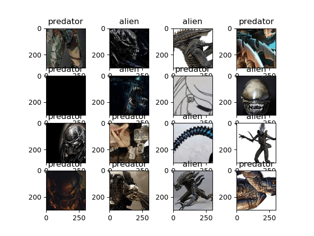
The collection is deliberately small, and a sample of the pictures it contains is shown below.

Source: Alien vs. Predator Kaggle
Next in this PyTorch Transfer Learning tutorial, you will learn how to apply Transfer Learning with PyTorch step by step.
How to Use Transfer Learning?
Here is a step by step process on how to use Transfer Learning for Deep Learning with PyTorch:
Step 1) Load the Data
The first step is to load the data and apply some transformations to the images so that they match the requirements of the network.
You will load the data from a folder with torchvision.datasets. The module iterates over the folder to split the data into train and validation sets. The transformation pipeline used here crops the images from the centre, converts them to a tensor, and normalises them for Deep Learning.
from __future__ import print_function, division
import os
import time
import torch
import torchvision
from torchvision import datasets, models, transforms
import torch.optim as optim
import numpy as np
import matplotlib.pyplot as plt

data_dir = "alien_pred"
input_shape = 224
mean = [0.5, 0.5, 0.5]
std = [0.5, 0.5, 0.5]

#data transformation
data_transforms = {
   'train': transforms.Compose([
       transforms.CenterCrop(input_shape),
       transforms.ToTensor(),
       transforms.Normalize(mean, std)
   ]),
   'validation': transforms.Compose([
       transforms.CenterCrop(input_shape),
       transforms.ToTensor(),
       transforms.Normalize(mean, std)
   ]),
}

image_datasets = {
   x: datasets.ImageFolder(
       os.path.join(data_dir, x),
       transform=data_transforms[x]
   )
   for x in ['train', 'validation']
}

dataloaders = {
   x: torch.utils.data.DataLoader(
       image_datasets[x], batch_size=32,
       shuffle=True, num_workers=4
   )
   for x in ['train', 'validation']
}

dataset_sizes = {x: len(image_datasets[x]) for x in ['train', 'validation']}

print(dataset_sizes)
class_names = image_datasets['train'].classes

device = torch.device("cuda:0" if torch.cuda.is_available() else "cpu")
Now visualise the dataset. The visualisation step takes the next batch of images and labels from the training data loader and displays them with Matplotlib.
images, labels = next(iter(dataloaders['train']))

rows = 4
columns = 4
fig=plt.figure()
for i in range(16):
   fig.add_subplot(rows, columns, i+1)
   plt.title(class_names[labels[i]])
   img = images[i].numpy().transpose((1, 2, 0))
   img = std * img + mean
   plt.imshow(img)
plt.show()
Running that snippet draws a four-by-four grid of training pictures, each one titled with the class name that the loader returned.
Step 2) Define Model
In this Deep Learning process, you will use VGG19 from the torchvision module.
You will use torchvision.models to load vgg19 with the pre-trained weights enabled. After that, you freeze the layers so that they are not trainable. You then modify the last layer with a Linear layer that fits the problem, which here means 2 classes. CrossEntropyLoss is used as the loss function, and the optimiser is SGD with a learning rate of 0.001 and a momentum of 0.9, as shown in the below PyTorch Transfer Learning example.
## Load the model based on VGG19
vgg_based = torchvision.models.vgg19(pretrained=True)

## freeze the layers
for param in vgg_based.parameters():
   param.requires_grad = False

# Modify the last layer
number_features = vgg_based.classifier[6].in_features
features = list(vgg_based.classifier.children())[:-1] # Remove last layer
features.extend([torch.nn.Linear(number_features, len(class_names))])
vgg_based.classifier = torch.nn.Sequential(*features)

vgg_based = vgg_based.to(device)

print(vgg_based)

criterion = torch.nn.CrossEntropyLoss()
optimizer_ft = optim.SGD(vgg_based.parameters(), lr=0.001, momentum=0.9)
Version note: the pretrained=True argument still works but has been superseded since torchvision 0.13 by the weights argument, so newer installs expect torchvision.models.vgg19(weights=VGG19_Weights.DEFAULT) and print a deprecation warning otherwise. Both forms load the same ImageNet weights.
The output model structure
Printing the model returns the full VGG19 graph. Read the last line of the classifier block to confirm the swap worked: it now produces 2 outputs instead of the 1,000 ImageNet classes.
VGG(
  (features): Sequential(
	(0): Conv2d(3, 64, kernel_size=(3, 3), stride=(1, 1), padding=(1, 1))
	(1): ReLU(inplace)
	(2): Conv2d(64, 64, kernel_size=(3, 3), stride=(1, 1), padding=(1, 1))
	(3): ReLU(inplace)
	(4): MaxPool2d(kernel_size=2, stride=2, padding=0, dilation=1, ceil_mode=False)
	(5): Conv2d(64, 128, kernel_size=(3, 3), stride=(1, 1), padding=(1, 1))
	(6): ReLU(inplace)
	(7): Conv2d(128, 128, kernel_size=(3, 3), stride=(1, 1), padding=(1, 1))
	(8): ReLU(inplace)
	(9): MaxPool2d(kernel_size=2, stride=2, padding=0, dilation=1, ceil_mode=False)
	(10): Conv2d(128, 256, kernel_size=(3, 3), stride=(1, 1), padding=(1, 1))
	(11): ReLU(inplace)
	(12): Conv2d(256, 256, kernel_size=(3, 3), stride=(1, 1), padding=(1, 1))
	(13): ReLU(inplace)
	(14): Conv2d(256, 256, kernel_size=(3, 3), stride=(1, 1), padding=(1, 1))
	(15): ReLU(inplace)
	(16): Conv2d(256, 256, kernel_size=(3, 3), stride=(1, 1), padding=(1, 1))
	(17): ReLU(inplace)
	(18): MaxPool2d(kernel_size=2, stride=2, padding=0, dilation=1, ceil_mode=False)
	(19): Conv2d(256, 512, kernel_size=(3, 3), stride=(1, 1), padding=(1, 1))
	(20): ReLU(inplace)
	(21): Conv2d(512, 512, kernel_size=(3, 3), stride=(1, 1), padding=(1, 1))
	(22): ReLU(inplace)
	(23): Conv2d(512, 512, kernel_size=(3, 3), stride=(1, 1), padding=(1, 1))
	(24): ReLU(inplace)
	(25): Conv2d(512, 512, kernel_size=(3, 3), stride=(1, 1), padding=(1, 1))
	(26): ReLU(inplace)
	(27): MaxPool2d(kernel_size=2, stride=2, padding=0, dilation=1, ceil_mode=False)
	(28): Conv2d(512, 512, kernel_size=(3, 3), stride=(1, 1), padding=(1, 1))
	(29): ReLU(inplace)
	(30): Conv2d(512, 512, kernel_size=(3, 3), stride=(1, 1), padding=(1, 1))
	(31): ReLU(inplace)
	(32): Conv2d(512, 512, kernel_size=(3, 3), stride=(1, 1), padding=(1, 1))
	(33): ReLU(inplace)
	(34): Conv2d(512, 512, kernel_size=(3, 3), stride=(1, 1), padding=(1, 1))
	(35): ReLU(inplace)
	(36): MaxPool2d(kernel_size=2, stride=2, padding=0, dilation=1, ceil_mode=False)
  )
  (classifier): Sequential(
	(0): Linear(in_features=25088, out_features=4096, bias=True)
	(1): ReLU(inplace)
	(2): Dropout(p=0.5)
	(3): Linear(in_features=4096, out_features=4096, bias=True)
	(4): ReLU(inplace)
	(5): Dropout(p=0.5)
	(6): Linear(in_features=4096, out_features=2, bias=True)
  )
)
Step 3) Train and Test Model
We will use some of the functions from this PyTorch Tutorial to help us train and evaluate our model.
def train_model(model, criterion, optimizer, num_epochs=25):
   since = time.time()

   for epoch in range(num_epochs):
       print('Epoch {}/{}'.format(epoch, num_epochs - 1))
       print('-' * 10)

       #set model to trainable
       # model.train()

       train_loss = 0

       # Iterate over data.
       for i, data in enumerate(dataloaders['train']):
           inputs , labels = data
           inputs = inputs.to(device)
           labels = labels.to(device)

           optimizer.zero_grad()

           with torch.set_grad_enabled(True):
               outputs  = model(inputs)
               loss = criterion(outputs, labels)

           loss.backward()
           optimizer.step()

           train_loss += loss.item() * inputs.size(0)

           print('{} Loss: {:.4f}'.format(
               'train', train_loss / dataset_sizes['train']))

   time_elapsed = time.time() - since
   print('Training complete in {:.0f}m {:.0f}s'.format(
       time_elapsed // 60, time_elapsed % 60))

   return model

def visualize_model(model, num_images=6):
   was_training = model.training
   model.eval()
   images_so_far = 0
   fig = plt.figure()

   with torch.no_grad():
       for i, (inputs, labels) in enumerate(dataloaders['validation']):
           inputs = inputs.to(device)
           labels = labels.to(device)

           outputs = model(inputs)
           _, preds = torch.max(outputs, 1)

           for j in range(inputs.size()[0]):
               images_so_far += 1
               ax = plt.subplot(num_images//2, 2, images_so_far)
               ax.axis('off')
               ax.set_title('predicted: {} truth: {}'.format(class_names[preds[j]], class_names[labels[j]]))
               img = inputs.cpu().data[j].numpy().transpose((1, 2, 0))
               img = std * img + mean
               ax.imshow(img)

               if images_so_far == num_images:
                   model.train(mode=was_training)
                   return
       model.train(mode=was_training)
Finally in this Transfer Learning in PyTorch example, start the training process with the number of epochs set to 25 and evaluate the network afterwards. At each training step the model takes the input and predicts the output. The prediction is passed to the criterion to calculate the loss, backpropagation calculates the gradients, and the optimiser updates the weights with autograd.
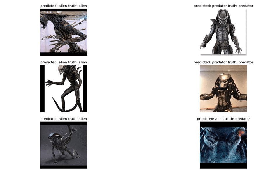
In the visualisation function, the trained network is tested with a batch of images to predict the labels, and the result is drawn with Matplotlib.
vgg_based = train_model(vgg_based, criterion, optimizer_ft, num_epochs=25)

visualize_model(vgg_based)

plt.show()
Step 4) Results
The accuracy reported for this run is 92%. The log printed at the end of training shows the running loss for the last two epochs together with the total training time.
Epoch 23/24
----------
train Loss: 0.0044
train Loss: 0.0078
train Loss: 0.0141
train Loss: 0.0221
train Loss: 0.0306
train Loss: 0.0336
train Loss: 0.0442
train Loss: 0.0482
train Loss: 0.0557
train Loss: 0.0643
train Loss: 0.0763
train Loss: 0.0779
train Loss: 0.0843
train Loss: 0.0910
train Loss: 0.0990
train Loss: 0.1063
train Loss: 0.1133
train Loss: 0.1220
train Loss: 0.1344
train Loss: 0.1382
train Loss: 0.1429
train Loss: 0.1500
Epoch 24/24
----------
train Loss: 0.0076
train Loss: 0.0115
train Loss: 0.0185
train Loss: 0.0277
train Loss: 0.0345
train Loss: 0.0420
train Loss: 0.0450
train Loss: 0.0490
train Loss: 0.0644
train Loss: 0.0755
train Loss: 0.0813
train Loss: 0.0868
train Loss: 0.0916
train Loss: 0.0980
train Loss: 0.1008
train Loss: 0.1101
train Loss: 0.1176
train Loss: 0.1282
train Loss: 0.1323
train Loss: 0.1397
train Loss: 0.1436
train Loss: 0.1467
Training complete in 2m 47s
The predictions of the model are then visualised with Matplotlib, as shown below.
Common Transfer Learning Errors and How to Fix Them
Most failures in a transfer learning script are mechanical rather than mathematical. These are the ones that stop the code above from running, and what each one means.
- Size mismatch in the final layer: the replaced Linear layer must accept the in_features reported by the original classifier and emit exactly len(class_names) outputs. Printing the model, as in Step 2, is the fastest way to confirm both numbers.
- The backbone was never frozen: if requires_grad is left at True, every VGG19 parameter is updated and the run slows to a crawl on a CPU. Set it to False before the classifier is replaced.
- Normalisation mismatch: the mean and standard deviation used in transforms.Normalize must be the same values at training and inference time, otherwise the predictions drift for no visible reason.
- Deprecated weights argument: on torchvision 0.13 and later, pretrained=True raises a deprecation warning and the weights enum is preferred.
- num_workers on Windows and notebooks: a DataLoader with num_workers=4 needs the entry point guarded, so set num_workers=0 if Python raises a spawn or pickling error.
- Evaluating in training mode: call model.eval() before scoring so that Dropout and BatchNorm behave deterministically, and switch back with model.train() afterwards.
