R Stepwise & Multiple Linear Regression [Step by Step Example]
Simple Linear Regression in R
Linear regression answers a simple question: Can you measure an exact relationship between one target variables and a set of predictors?
The simplest of probabilistic model is the straight line model:
![]()
where
- y = Dependent variable
- x = Independent variable
-
 = random error component
 -
 = intercept
 -
 = Coefficient of x
Consider the following plot:
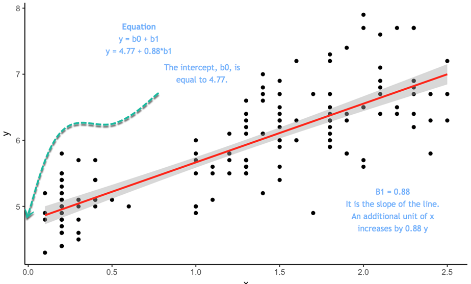
The equation is ![]() is the intercept. If x equals to 0, y will be equal to the intercept, 4.77. is the slope of the line. It tells in which proportion y varies when x varies.
is the intercept. If x equals to 0, y will be equal to the intercept, 4.77. is the slope of the line. It tells in which proportion y varies when x varies.
To estimate the optimal values of ![]() and
and ![]() , you use a method called Ordinary Least Squares (OLS). This method tries to find the parameters that minimize the sum of the squared errors, that is the vertical distance between the predicted y values and the actual y values. The difference is known as the error term.
, you use a method called Ordinary Least Squares (OLS). This method tries to find the parameters that minimize the sum of the squared errors, that is the vertical distance between the predicted y values and the actual y values. The difference is known as the error term.
Before you estimate the model, you can determine whether a linear relationship between y and x is plausible by plotting a scatterplot.
Scatterplot
We will use a very simple dataset to explain the concept of simple linear regression. We will import the Average Heights and weights for American Women. The dataset contains 15 observations. You want to measure whether Heights are positively correlated with weights.
library(ggplot2)
path <- 'https://raw.githubusercontent.com/guru99-edu/R-Programming/master/women.csv'
df <-read.csv(path)
ggplot(df,aes(x=height, y =  weight))+
geom_point()
Output:

The scatterplot suggests a general tendency for y to increase as x increases. In the next step, you will measure by how much increases for each additional .
Least Squares Estimates
In a simple OLS regression, the computation of ![]() and
and ![]() is straightforward. The goal is not to show the derivation in this tutorial. You will only write the formula.
is straightforward. The goal is not to show the derivation in this tutorial. You will only write the formula.
You want to estimate: ![]()
The goal of the OLS regression is to minimize the following equation:
![]()
where
![]() is the actual value and
is the actual value and ![]() is the predicted value.
is the predicted value.
The solution for ![]() is
is ![]()
Note that ![]() means the average value of x
means the average value of x
The solution for ![]() is
is ![]()
In R, you can use the cov()and var()function to estimate ![]() and you can use the mean() function to estimate
and you can use the mean() function to estimate ![]()
beta <- cov(df$height, df$weight) / var (df$height)
beta
Output:
##[1] 3.45
alpha <- mean(df$weight) - beta * mean(df$height)
alpha
Output:
## [1] -87.51667
The beta coefficient implies that for each additional height, the weight increases by 3.45.
Estimating simple linear equation manually is not ideal. R provides a suitable function to estimate these parameters. You will see this function shortly. Before that, we will introduce how to compute by hand a simple linear regression model. In your journey of data scientist, you will barely or never estimate a simple linear model. In most situation, regression tasks are performed on a lot of estimators.
Multiple Linear Regression in R
More practical applications of regression analysis employ models that are more complex than the simple straight-line model. The probabilistic model that includes more than one independent variable is called multiple regression models. The general form of this model is:
![]()
In matrix notation, you can rewrite the model:
The dependent variable y is now a function of k independent variables. The value of the coefficient ![]() determines the contribution of the independent variable
determines the contribution of the independent variable ![]() and
and ![]() .
.
We briefly introduce the assumption we made about the random error ![]() of the OLS:
of the OLS:
- Mean equal to 0
- Variance equal to

- Normal distribution
- Random errors are independent (in a probabilistic sense)
You need to solve for ![]() , the vector of regression coefficients that minimise the sum of the squared errors between the predicted and actual y values.
, the vector of regression coefficients that minimise the sum of the squared errors between the predicted and actual y values.
The closed-form solution is:
![]()
with:
- indicates the transpose of the matrix X
 indicates the invertible matrix
We use the mtcars dataset. You are already familiar with the dataset. Our goal is to predict the mile per gallon over a set of features.
Continuous Variables in R
For now, you will only use the continuous variables and put aside categorical features. The variable am is a binary variable taking the value of 1 if the transmission is manual and 0 for automatic cars; vs is also a binary variable.
library(dplyr)
df <- mtcars % > %
select(-c(am, vs, cyl, gear, carb))
glimpse(df)
Output:
## Observations: 32
## Variables: 6
## $ mpg  <dbl> 21.0, 21.0, 22.8, 21.4, 18.7, 18.1, 14.3, 24.4, 22.8, 19....
## $ disp <dbl> 160.0, 160.0, 108.0, 258.0, 360.0, 225.0, 360.0, 146.7, 1...
## $ hp   <dbl> 110, 110, 93, 110, 175, 105, 245, 62, 95, 123, 123, 180, ...
## $ drat <dbl> 3.90, 3.90, 3.85, 3.08, 3.15, 2.76, 3.21, 3.69, 3.92, 3.9...
## $ wt   <dbl> 2.620, 2.875, 2.320, 3.215, 3.440, 3.460, 3.570, 3.190, 3...
## $ qsec <dbl> 16.46, 17.02, 18.61, 19.44, 17.02, 20.22, 15.84, 20.00, 2...
You can use the lm() function to compute the parameters. The basic syntax of this function is:
lm(formula, data, subset)
Arguments:
	-formula: The equation you want to estimate
	-data: The dataset used
	-subset: Estimate the model on a subset of the dataset
Remember an equation is of the following form
![]()
in R
- The symbol = is replaced by ~
- Each x is replaced by the variable name
- If you want to drop the constant, add -1 at the end of the formula
Example:
You want to estimate the weight of individuals based on their height and revenue. The equation is
![]()
The equation in R is written as follow:
y ~ X1+ X2+…+Xn # With intercept
So for our example:
- Weigh ~ height + revenue
Your objective is to estimate the mile per gallon based on a set of variables. The equation to estimate is:
![]()
You will estimate your first linear regression and store the result in the fit object.
model <- mpg~.disp + hp + drat + wt
fit <- lm(model, df)
fit
Code Explanation
- model <- mpg ~. disp + hp + drat+ wt: Store the model to estimate
- lm(model, df): Estimate the model with the data frame df
##
## Call:
## lm(formula = model, data = df)
##
## Coefficients:
## (Intercept)         disp           hp         drat           wt
##    16.53357      0.00872     -0.02060      2.01577     -4.38546
##        qsec
##     0.64015
The output does not provide enough information about the quality of the fit. You can access more details such as the significance of the coefficients, the degree of freedom and the shape of the residuals with the summary() function.
summary(fit)
Output:
## return the p-value and coefficient
##
## Call:
## lm(formula = model, data = df)
##
## Residuals:
##     Min      1Q  Median      3Q     Max
## -3.5404 -1.6701 -0.4264  1.1320  5.4996
##
## Coefficients:
##             Estimate Std. Error t value Pr(>|t|)
## (Intercept) 16.53357   10.96423   1.508  0.14362
## disp         0.00872    0.01119   0.779  0.44281
## hp          -0.02060    0.01528  -1.348  0.18936
## drat         2.01578    1.30946   1.539  0.13579
## wt          -4.38546    1.24343  -3.527  0.00158 **
## qsec         0.64015    0.45934   1.394  0.17523
## ---
## Signif. codes:  0 '***' 0.001 '**' 0.01 '*' 0.05 '.' 0.1 ' ' 1
##
## Residual standard error: 2.558 on 26 degrees of freedom
## Multiple R-squared:  0.8489, Adjusted R-squared:  0.8199
## F-statistic: 29.22 on 5 and 26 DF, p-value: 6.892e-10
Inference from the above table output
- The above table proves that there is a strong negative relationship between wt and mileage and positive relationship with drat.
- Only the variable wt has a statistical impact on mpg. Remember, to test a hypothesis in statistic, we use:
- H0: No statistical impact
- H3: The predictor has a meaningful impact on y
- If the p value is lower than 0.05, it indicates the variable is statistically significant
- Adjusted R-squared: Variance explained by the model. In your model, the model explained 82 percent of the variance of y. R squared is always between 0 and 1. The higher the better
You can run the ANOVA test to estimate the effect of each feature on the variances with the anova() function.
anova(fit)
Output:
## Analysis of Variance Table
##
## Response: mpg
##           Df Sum Sq Mean Sq  F value   Pr(>F)
## disp       1 808.89  808.89 123.6185 2.23e-11 ***
## hp         1  33.67   33.67   5.1449 0.031854 *
## drat       1  30.15   30.15   4.6073 0.041340 *
## wt         1  70.51   70.51  10.7754 0.002933 **
## qsec       1  12.71   12.71   1.9422 0.175233
## Residuals 26 170.13    6.54
## ---
## Signif. codes:  0 '***' 0.001 '**' 0.01 '*' 0.05 '.' 0.1 ' ' 1
A more conventional way to estimate the model performance is to display the residual against different measures.
You can use the plot() function to show four graphs:
– Residuals vs Fitted values
– Normal Q-Q plot: Theoretical Quartile vs Standardized residuals
– Scale-Location: Fitted values vs Square roots of the standardised residuals
– Residuals vs Leverage: Leverage vs Standardized residuals
You add the code par(mfrow=c(2,2)) before plot(fit). If you don’t add this line of code, R prompts you to hit the enter command to display the next graph.
par(mfrow=(2,2))
Code Explanation
- (mfrow=c(2,2)): return a window with the four graphs side by side.
- The first 2 adds the number of rows
- The second 2 adds the number of columns.
- If you write (mfrow=c(3,2)): you will create a 3 rows 2 columns window
plot(fit)
Output:

The lm() formula returns a list containing a lot of useful information. You can access them with the fit object you have created, followed by the $ sign and the information you want to extract.
– coefficients: `fit$coefficients`
– residuals: `fit$residuals`
– fitted value: `fit$fitted.values`
Factors Regression in R
In the last model estimation, you regress mpg on continuous variables only. It is straightforward to add factor variables to the model. You add the variable am to your model. It is important to be sure the variable is a factor level and not continuous.
df <- mtcars % > %
mutate(cyl = factor(cyl),
    vs = factor(vs),
    am = factor(am),
    gear = factor(gear),
    carb = factor(carb))
summary(lm(model, df))
Output:
##
## Call:
## lm(formula = model, data = df)
##
## Residuals:
##     Min      1Q  Median      3Q     Max
## -3.5087 -1.3584 -0.0948  0.7745  4.6251
##
## Coefficients:
##             Estimate Std. Error t value Pr(>|t|)
## (Intercept) 23.87913   20.06582   1.190   0.2525
## cyl6        -2.64870    3.04089  -0.871   0.3975
## cyl8        -0.33616    7.15954  -0.047   0.9632
## disp         0.03555    0.03190   1.114   0.2827
## hp          -0.07051    0.03943  -1.788   0.0939 .
## drat         1.18283    2.48348   0.476   0.6407
## wt          -4.52978    2.53875  -1.784   0.0946 .
## qsec         0.36784    0.93540   0.393   0.6997
## vs1          1.93085    2.87126   0.672   0.5115
## am1          1.21212    3.21355   0.377   0.7113
## gear4        1.11435    3.79952   0.293   0.7733
## gear5        2.52840    3.73636   0.677   0.5089
## carb2       -0.97935    2.31797  -0.423   0.6787
## carb3        2.99964    4.29355   0.699   0.4955
## carb4        1.09142    4.44962   0.245   0.8096
## carb6        4.47757    6.38406   0.701   0.4938
## carb8        7.25041    8.36057   0.867   0.3995
## ---
## Signif. codes:  0 '***' 0.001 '**' 0.01 '*' 0.05 '.' 0.1 ' ' 1
##
## Residual standard error: 2.833 on 15 degrees of freedom
## Multiple R-squared:  0.8931, Adjusted R-squared:  0.779
## F-statistic:  7.83 on 16 and 15 DF,  p-value: 0.000124
R uses the first factor level as a base group. You need to compare the coefficients of the other group against the base group.
Stepwise Linear Regression in R
The last part of this tutorial deals with the stepwise regression algorithm. The purpose of this algorithm is to add and remove potential candidates in the models and keep those who have a significant impact on the dependent variable. This algorithm is meaningful when the dataset contains a large list of predictors. You don’t need to manually add and remove the independent variables. The stepwise regression is built to select the best candidates to fit the model.
Let’s see in action how it works. You use the mtcars dataset with the continuous variables only for pedagogical illustration. Before you begin analysis, its good to establish variations between the data with a correlation matrix. The GGally library is an extension of ggplot2.
The library includes different functions to show summary statistics such as correlation and distribution of all the variables in a matrix. We will use the ggscatmat function, but you can refer to the vignette for more information about the GGally library.
The basic syntax for ggscatmat() is:
ggscatmat(df, columns = 1:ncol(df), corMethod = "pearson")
arguments:
-df:  A matrix of continuous variables
-columns: Pick up the columns to use in the function. By default, all columns are used
-corMethod: Define the function to compute the correlation between variable. By default, the algorithm uses the Pearson formula
You display the correlation for all your variables and decides which one will be the best candidates for the first step of the stepwise regression. There are some strong correlations between your variables and the dependent variable, mpg.
library(GGally)
df <- mtcars % > %
	select(-c(am, vs, cyl, gear, carb))
ggscatmat(df, columns = 1: ncol(df))
Output:

Stepwise Regression Step by Step Example
Variables selection is an important part to fit a model. The stepwise regression will perform the searching process automatically. To estimate how many possible choices there are in the dataset, you compute ![]() with k is the number of predictors. The amount of possibilities grows bigger with the number of independent variables. That’s why you need to have an automatic search.
with k is the number of predictors. The amount of possibilities grows bigger with the number of independent variables. That’s why you need to have an automatic search.
You need to install the olsrr package from CRAN. The package is not available yet in Anaconda. Hence, you install it directly from the command line:
install.packages("olsrr")
You can plot all the subsets of possibilities with the fit criteria (i.e. R-square, Adjusted R-square, Bayesian criteria). The model with the lowest AIC criteria will be the final model.
library(olsrr)
model <- mpg~.
fit <- lm(model, df)
test <- ols_all_subset(fit)
plot(test)
Code Explanation
- mpg ~.: Construct the model to estimate
- lm(model, df): Run the OLS model
- ols_all_subset(fit): Construct the graphs with the relevant statistical information
- plot(test): Plot the graphs
Output:

Linear regression models use the t-test to estimate the statistical impact of an independent variable on the dependent variable. Researchers set the maximum threshold at 10 percent, with lower values indicates a stronger statistical link. The strategy of the stepwise regression is constructed around this test to add and remove potential candidates. The algorithm works as follow:

- Step 1: Regress each predictor on y separately. Namely, regress x_1 on y, x_2 on y to x_n. Store the p-value and keep the regressor with a p-value lower than a defined threshold (0.1 by default). The predictors with a significance lower than the threshold will be added to the final model. If no variable has a p-value lower than the entering threshold, then the algorithm stops, and you have your final model with a constant only.
- Step 2: Use the predictor with the lowest p-value and adds separately one variable. You regress a constant, the best predictor of step one and a third variable. You add to the stepwise model, the new predictors with a value lower than the entering threshold. If no variable has a p-value lower than 0.1, then the algorithm stops, and you have your final model with one predictor only. You regress the stepwise model to check the significance of the step 1 best predictors. If it is higher than the removing threshold, you keep it in the stepwise model. Otherwise, you exclude it.
- Step 3: You replicate step 2 on the new best stepwise model. The algorithm adds predictors to the stepwise model based on the entering values and excludes predictor from the stepwise model if it does not satisfy the excluding threshold.
- The algorithm keeps on going until no variable can be added or excluded.
You can perform the algorithm with the function ols_stepwise() from the olsrr package.
ols_stepwise(fit, pent = 0.1, prem = 0.3, details = FALSE)

arguments:
-fit:  Model to fit. Need to use `lm()`before to run `ols_stepwise()
-pent: Threshold of the p-value used to enter a variable into the stepwise model. By default, 0.1
-prem: Threshold of the p-value used to exclude a variable into the stepwise model. By default, 0.3
-details: Print the details of each step
Before that, we show you the steps of the algorithm. Below is a table with the dependent and independent variables:
| Dependent variable | Independent variables |
|---|---|
| mpg | disp |
| hp | |
| drat | |
| wt | |
| qsec |
Start
To begin with, the algorithm starts by running the model on each independent variable separately. The table shows the p-value for each model.
## [[1]]
##  (Intercept)         disp
## 3.576586e-21 9.380327e-10
##
## [[2]]
##  (Intercept)           hp
## 6.642736e-18 1.787835e-07
##
## [[3]]
##  (Intercept)         drat
## 0.1796390847 0.0000177624
##
## [[4]]
##  (Intercept)           wt
## 8.241799e-19 1.293959e-10
##
## [[5]
## (Intercept)        qsec
##  0.61385436  0.01708199
To enter the model, the algorithm keeps the variable with the lowest p-value. From the above output, it is wt
Step 1
In the first step, the algorithm runs mpg on wt and the other variables independently.
## [[1]]
##  (Intercept)           wt         disp
## 4.910746e-16 7.430725e-03 6.361981e-02
##
## [[2]]
##  (Intercept)           wt           hp
## 2.565459e-20 1.119647e-06 1.451229e-03
##
## [[3]]
##  (Intercept)           wt         drat
## 2.737824e-04 1.589075e-06 3.308544e-01
##
## [[4]]
##  (Intercept)           wt         qsec
## 7.650466e-04 2.518948e-11 1.499883e-03
Each variable is a potential candidate to enter the final model. However, the algorithm keeps only the variable with the lower p-value. It turns out hp has a slighlty lower p-value than qsec. Therefore, hp enters the final model
Step 2
The algorithm repeats the first step but this time with two independent variables in the final model.
## [[1]]
##  (Intercept)           wt           hp         disp
## 1.161936e-16 1.330991e-03 1.097103e-02 9.285070e-01
##
## [[2]]
##  (Intercept)           wt           hp         drat
## 5.133678e-05 3.642961e-04 1.178415e-03 1.987554e-01
##
## [[3]]
##  (Intercept)           wt           hp         qsec
## 2.784556e-03 3.217222e-06 2.441762e-01 2.546284e-01
None of the variables that entered the final model has a p-value sufficiently low. The algorithm stops here; we have the final model:
##
## Call:
## lm(formula = mpg ~ wt + hp, data = df)
##
## Residuals:
##    Min     1Q Median     3Q    Max
## -3.941 -1.600 -0.182  1.050  5.854
##
## Coefficients:
##             Estimate Std. Error t value Pr(>|t|)
## (Intercept) 37.22727    1.59879  23.285  < 2e-16 ***
## wt          -3.87783    0.63273  -6.129 1.12e-06 ***
## hp          -0.03177    0.00903  -3.519  0.00145 **
## ---
## Signif. codes:  0 '***' 0.001 '**' 0.01 '*' 0.05 '.' 0.1 ' ' 1
##
## Residual standard error: 2.593 on 29 degrees of freedom
## Multiple R-squared:  0.8268, Adjusted R-squared:  0.8148
## F-statistic: 69.21 on 2 and 29 DF,  p-value: 9.109e-12
You can use the function ols_stepwise() to compare the results.
stp_s <-ols_stepwise(fit, details=TRUE)
Output:
The algorithm founds a solution after 2 steps, and return the same output as we had before.
At the end, you can say the models is explained by two variables and an intercept. Mile per gallon is negatively correlated with Gross horsepower and Weight
## You are selecting variables based on p value...
## 1 variable(s) added....
## Variable Selection Procedure
##  Dependent Variable: mpg
##
##  Stepwise Selection: Step 1
##
##  Variable wt Entered
##
##                         Model Summary
## --------------------------------------------------------------
## R                       0.868       RMSE                3.046
## R-Squared               0.753       Coef. Var          15.161
## Adj. R-Squared          0.745       MSE                 9.277
## Pred R-Squared          0.709       MAE                 2.341
## --------------------------------------------------------------
##  RMSE: Root Mean Square Error
##  MSE: Mean Square Error
##  MAE: Mean Absolute Error
##		ANOVA
## --------------------------------------------------------------------
##                 Sum of
##                Squares        DF    Mean Square      F         Sig.
## --------------------------------------------------------------------
## Regression     847.725         1        847.725    91.375    0.0000
## Residual       278.322        30          9.277
## Total         1126.047        31
## --------------------------------------------------------------------
##
##                                   Parameter Estimates
## ----------------------------------------------------------------------------------------
##       model      Beta    Std. Error    Std. Beta      t        Sig      lower     upper
## ----------------------------------------------------------------------------------------
## (Intercept)    37.285         1.878                 19.858    0.000    33.450    41.120
##          wt    -5.344         0.559       -0.868    -9.559    0.000    -6.486    -4.203
## ----------------------------------------------------------------------------------------
## 1 variable(s) added...
## Stepwise Selection: Step 2
##
##  Variable hp Entered
##
##                         Model Summary
## --------------------------------------------------------------
## R                       0.909       RMSE                2.593
## R-Squared               0.827       Coef. Var          12.909
## Adj. R-Squared          0.815       MSE                 6.726
## Pred R-Squared          0.781       MAE                 1.901
## --------------------------------------------------------------
##  RMSE: Root Mean Square Error
##  MSE: Mean Square Error
##  MAE: Mean Absolute Error
##			ANOVA
## --------------------------------------------------------------------
##                 Sum of
##                Squares        DF    Mean Square      F         Sig.
## --------------------------------------------------------------------
## Regression     930.999         2        465.500    69.211    0.0000
## Residual       195.048        29          6.726
## Total         1126.047        31
## --------------------------------------------------------------------
##
##                                   Parameter Estimates
## ----------------------------------------------------------------------------------------
##       model      Beta    Std. Error    Std. Beta      t        Sig      lower     upper
## ----------------------------------------------------------------------------------------
## (Intercept)    37.227         1.599                 23.285    0.000    33.957    40.497
##          wt    -3.878         0.633       -0.630    -6.129    0.000    -5.172    -2.584
##          hp    -0.032         0.009       -0.361    -3.519    0.001    -0.050    -0.013
## ----------------------------------------------------------------------------------------
## No more variables to be added or removed.
Machine Learning
Machine Learning is becoming widespread among data scientist and is deployed in hundreds of products you use daily. One of the first ML application was spam filter.
Following are other application of Machine Learning-
- Identification of unwanted spam messages in email
- Segmentation of customer behavior for targeted advertising
- Reduction of fraudulent credit card transactions
- Optimization of energy use in home and office building
- Facial recognition
Supervised Learning
In Supervised Learning, the training data you feed to the algorithm includes a label.
Classification is probably the most used supervised learning technique. One of the first classification task researchers tackled was the spam filter. The objective of the learning is to predict whether an email is classified as spam or ham (good email). The machine, after the training step, can detect the class of email.
Regressions are commonly used in the machine learning field to predict continuous value. Regression task can predict the value of a dependent variable based on a set of independent variables (also called predictors or regressors). For instance, linear regressions can predict a stock price, weather forecast, sales and so on.
Here is the list of some fundamental supervised learning algorithms.
- Linear regression
- Logistic regression
- Nearest Neighbors
- Support Vector Machine (SVM)
- Decision trees and Random Forest
- Neural Networks
Unsupervised Learning
In Unsupervised Learning, the training data is unlabeled. The system tries to learn without a reference. Below is a list of unsupervised learning algorithms.
- K-mean
- Hierarchical Cluster Analysis
- Expectation Maximization
- Visualization and dimensionality reduction
- Principal Component Analysis
- Kernel PCA
- Locally-Linear Embedding
Summary
- Linear regression answers a simple question: Can you measure an exact relationship between one target variables and a set of predictors?
- Ordinary Least Squares method tries to find the parameters that minimize the sum of the squared errors, that is the vertical distance between the predicted y values and the actual y values.
- The probabilistic model that includes more than one independent variable is called multiple regression models.
- The purpose of Stepwise Linear Regression algorithm is to add and remove potential candidates in the models and keep those who have a significant impact on the dependent variable.
- Variables selection is an important part to fit a model. The stepwise regression performs the searching process automatically.
Ordinary least squared regression can be summarized in the table below:
| Library | Objective | Function | Arguments |
|---|---|---|---|
| base | Compute a linear regression | lm() | formula, data |
| base | Summarize model | summarize() | fit |
| base | Exctract coefficients | lm()$coefficient | |
| base | Exctract residuals | lm()$residuals | |
| base | Exctract fitted value | lm()$fitted.values | |
| olsrr | Run stepwise regression | ols_stepwise() | fit, pent = 0.1, prem = 0.3, details = FALSE |
Note: Remember to transform categorical variable in factor before to fit the model.