
ANOVA in R: One-Way & Two-Way Test with Examples
 Editorial Team
⚡ Smart Summary
ANOVA in R compares the means of three or more groups by splitting total variation into between-group and within-group components. This walkthrough runs one-way and two-way tests on the poisons dataset, checks assumptions, and isolates differing pairs with Tukey HSD.

What is ANOVA?
Analysis of Variance (ANOVA) is a statistical technique used to compare the means of two or more groups. The test works by splitting the total variation in a measurement into the part explained by group membership and the part left over as random noise. ANOVA in R therefore tells you whether at least one group mean differs from the others, not which one. It is a direct extension of the t-test to situations where the factor variable has more than two levels.
Before running a test, it helps to know which member of the ANOVA family fits your design.
Types of ANOVA Tests in R
“ANOVA” is a family of tests rather than a single procedure. Choosing the right member depends on how many factors you have and how the data were collected.
| Test | When to use it | R call |
|---|---|---|
| One-way ANOVA | One factor with three or more levels | aov(y ~ x, data = df) |
| Two-way ANOVA | Two independent factors | aov(y ~ x1 + x2, data = df) |
| Two-way with interaction | The effect of one factor depends on the other | aov(y ~ x1 * x2, data = df) |
| Repeated measures ANOVA | The same subjects measured more than once | aov(y ~ x + Error(subject/x)) |
| ANCOVA | A continuous covariate must be controlled for | aov(y ~ x + covariate, data = df) |
| MANOVA | Two or more response variables at once | manova(cbind(y1, y2) ~ x) |
This tutorial covers the first three. The remaining variants use the same aov() interface, so once you can read one output table you can read them all.
ANOVA vs T-Test in R: Key Differences
Both tests compare means, so it is worth being precise about where one replaces the other.
| Criteria | T-Test | ANOVA |
|---|---|---|
| Number of groups | Exactly two | Two or more |
| Test statistic | t | F, equal to t squared when there are two groups |
| Result | Names the direction of the difference | Only reports that a difference exists |
| Follow-up needed | None | Post hoc test such as Tukey HSD |
| R function | t.test() | aov() |
The temptation with three groups is to run three separate t-tests. Resist it. Each test carries its own 5 percent error rate, so three comparisons push the chance of a false positive to roughly 14 percent. ANOVA answers the same question with a single test, and Tukey HSD then handles the pairwise detail with the error rate held in check. For the two-group case, see the t-test tutorial.
One-way ANOVA
There are many situations where you need to compare the mean between multiple groups. For instance, the marketing department wants to know if three teams have the same sales performance.
- Team: 3 level factor: A, B, and C
- Sale: A measure of performance
The ANOVA test can tell if the three groups have similar performances.
To clarify if the data comes from the same population, you can perform a one-way analysis of variance (one-way ANOVA hereafter). Like any other statistical test, it gives evidence about whether the H0 hypothesis can be rejected. Note that failing to reject H0 is not the same as proving it true.
Hypothesis in one-way ANOVA test
- H0: The means between groups are identical
- H1: At least, the mean of one group is different
In other words, failing to reject H0 means there is not enough evidence to conclude that any group mean differs from the others.
This test is similar to the t-test, but ANOVA is the correct choice when there are more than two groups. With exactly two groups, the two tests are equivalent and the F-statistic equals the square of the t-statistic.
Assumptions
The one-way ANOVA rests on three conditions: observations are randomly sampled and independent of one another, the residuals within each group are approximately normally distributed, and the variance is the same in every group (homogeneity of variance). The section on checking assumptions below shows how to test each one in R.
Interpret ANOVA test
The F-statistic is used to test if the data are from significantly different populations, i.e., different sample means.
To compute the F-statistic, you need to divide the between-group variability over the within-group variability.
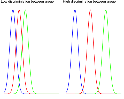
The between-group variability reflects how far each group mean sits from the overall mean. Compare the two graphs below to see the idea.
The left graph shows very little variation between the three groups, so all three group means sit close to the overall mean.
The right graph plots three distributions far apart with no overlap, so the gap between the overall mean and each group mean is large.
The within-group variability measures how far individual observations fall from the mean of their own group. Some points sit far from their group average, and the within-group term captures exactly that spread, which is the sampling error.
To understand visually the concept of within group variability, look at the graph below.
The left part plots the distribution of three different groups. You increased the spread of each sample and it is clear the individual variance is large. The F-statistic falls, so you would fail to reject the null hypothesis
The right part shows samples with the same means but much lower spread. That raises the F-statistic and points in favour of the alternative hypothesis.

You can use both measures to construct the F-statistics. It is very intuitive to understand the F-statistic. If the numerator increases, it means the between-group variability is high, and it is likely the groups in the sample are drawn from completely different distributions.
In other words, a low F-statistic indicates little or no meaningful difference between the group averages.
Example One way ANOVA Test
You will use the poison dataset to implement the one-way ANOVA test. The dataset contains 48 rows and 3 variables:
- Time: Survival time of the animal
- poison: Type of poison used: factor level: 1,2 and 3
- treat: Type of treatment used: factor level: 1,2 and 3
Before you start to compute the ANOVA test, you need to prepare the data as follow:
- Step 1: Import the data
- Step 2: Remove unnecessary variable
- Step 3: Convert the variable poison as ordered level
library(dplyr)
PATH <- "https://raw.githubusercontent.com/guru99-edu/R-Programming/master/poisons.csv"
df <- read.csv(PATH) %>%
select(-X) %>%
mutate(poison = factor(poison, ordered = TRUE))
glimpse(df)
Output:
## Observations: 48
## Variables: 3
## $ time   <dbl> 0.31, 0.45, 0.46, 0.43, 0.36, 0.29, 0.40, 0.23, 0.22, 0...
## $ poison <ord> 1, 1, 1, 1, 2, 2, 2, 2, 3, 3, 3, 3, 1, 1, 1, 1, 2, 2, 2...
## $ treat  <fctr> A, A, A, A, A, A, A, A, A, A, A, A, B, B, B, B, B, B, ...
Our objective is to test the following assumption:
- H0: There is no difference in survival time average between group
- H1: The survival time average is different for at least one group.
In other words, you want to know if there is a statistical difference between the mean of the survival time according to the type of poison given to the Guinea pig.
You will proceed as follow:
- Step 1: Check the format of the variable poison
- Step 2: Print the summary statistic: count, mean and standard deviation
- Step 3: Plot a box plot
- Step 4: Compute the one-way ANOVA test
- Step 5: Run a pairwise comparison with Tukey HSD
Step 1) Check the levels of poison with the code below. You should see three character values, because the mutate verb converted the column into an ordered factor.
levels(df$poison)
Output:
## [1] "1" "2" "3"
Step 2) You compute the mean and standard deviation.
df %>%
	group_by(poison) %>%
	summarise(
		count_poison = n(),
		mean_time = mean(time, na.rm = TRUE),
		sd_time = sd(time, na.rm = TRUE)
	)
Output:
##
# A tibble: 3 x 4
##   poison count_poison mean_time    sd_time
##    <ord>        <int>     <dbl>      <dbl>
## 1      1           16  0.617500 0.20942779
## 2      2           16  0.544375 0.28936641
## 3      3           16  0.276250 0.06227627
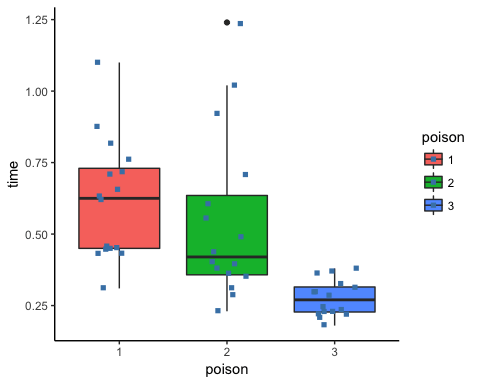
Step 3) In step three, you can graphically check if there is a difference between the distribution. Note that you include the jittered dot.
ggplot(df, aes(x = poison, y = time, fill = poison)) +
    geom_boxplot() +
    geom_jitter(shape = 15,
        color = "steelblue",
        position = position_jitter(0.21)) +
    theme_classic()
Output:
Step 4) You can run the one-way ANOVA test with the command aov. The basic syntax for an ANOVA test is:
aov(formula, data)
Arguments:
- formula: The equation you want to estimate
- data: The dataset used
The syntax of the formula is:
y ~ X1+ X2+...+Xn # X1 +  X2 +... refers to the independent variables
y ~ . # use all the remaining variables as independent variables
You can now answer the question: is there any difference in survival time between the guinea pigs, given the type of poison administered?
Store the model in an object and pass it to summary() to get a readable print of the results.
anova_one_way <- aov(time~poison, data = df)
summary(anova_one_way)
Code Explanation
- aov(time ~ poison, data = df): Run the ANOVA test with the following formula
- summary(anova_one_way): Print the summary of the test
Output:
##             Df Sum Sq Mean Sq F value   Pr(>F)
## poison       2  1.033  0.5165   11.79 7.66e-05 ***
## Residuals   45  1.972  0.0438
## ---
## Signif. codes:  0 '***' 0.001 '**' 0.01 '*' 0.05 '.' 0.1 ' ' 1
The p-value is 7.66e-05, far below the usual threshold of 0.05, and the three stars mark the strongest significance code. You can reject H0 and conclude that at least one poison group has a different mean survival time.
How to Check ANOVA Assumptions in R
An ANOVA p-value is only trustworthy when the three conditions listed earlier hold. Each one has a direct check in R, and all of them run on the fitted model object.
1. Independence of observations. This is a property of the study design, not of the data, so no test can rescue it. Each guinea pig must be measured once and assigned to its group at random. If the same subject appears in several rows, you need a repeated measures model instead.
2. Normality of residuals. ANOVA assumes the residuals, not the raw data, are approximately normal. Inspect the Q-Q plot and confirm with the Shapiro-Wilk test:
par(mfrow = c(2, 2))
plot(anova_one_way)          # four diagnostic plots

shapiro.test(residuals(anova_one_way))
Points hugging the diagonal of the Normal Q-Q plot indicate normal residuals. A Shapiro-Wilk p-value above 0.05 means you cannot reject normality.
3. Homogeneity of variance. Every group should show a similar spread. The Residuals vs Fitted plot should look like a flat band rather than a funnel. Confirm it with Levene’s test, which is more robust to non-normality than Bartlett’s:
library(car)
leveneTest(time ~ poison, data = df)

bartlett.test(time ~ poison, data = df)
A p-value above 0.05 supports equal variances.
What to do when an assumption fails. If variances are unequal, run oneway.test(time ~ poison, data = df, var.equal = FALSE), the Welch correction. If the residuals are clearly non-normal and the sample is small, switch to the Kruskal-Wallis rank test, kruskal.test(time ~ poison, data = df). With large balanced samples, ANOVA is fairly robust to moderate departures from normality, so a borderline Shapiro-Wilk result is rarely fatal.
Pairwise comparison
A significant F-test tells you that the group means are not all equal, but not which pair differs. The Tukey Honest Significant Difference test answers that by comparing every pair while controlling the family-wise error rate.
TukeyHSD(anova_one_way)
Output:

Read the output one row per pair. The diff column holds the difference between the two group means, lwr and upr bound the 95 percent confidence interval for that difference, and p adj is the p-value adjusted for multiple comparisons. A pair differs significantly when its interval excludes zero, equivalently when p adj is below 0.05. In this dataset the comparisons involving poison 3 are the significant ones, which matches the box plot: group 3 has a clearly lower mean survival time than groups 1 and 2, while groups 1 and 2 are statistically indistinguishable from each other.
Two-way ANOVA
A two-way ANOVA adds a second factor to the formula. It works exactly like the one-way test, only the formula changes:
y ~ x1 + x2
Here y is the quantitative response variable, while x1 and x2 are both categorical factors.
Hypothesis in two-way ANOVA test
- H0: The group means are equal for both factor variables
- H1: At least one group mean differs, for at least one of the two factors
You add the treat variable to the model. This variable records the treatment given to the guinea pig. The additive formula below tests whether each factor affects survival time on its own, after accounting for the other.
Adjust the code by adding treat alongside the first independent variable.
anova_two_way <- aov(time~poison + treat, data = df)
summary(anova_two_way)
Output:
##             Df Sum Sq Mean Sq F value  Pr(>F)
## poison       2 1.0330  0.5165   20.64 5.7e-07 ***
## treat        3 0.9212  0.3071   12.27 6.7e-06 ***
## Residuals   42 1.0509  0.0250
## ---
Both p-values (5.7e-07 for poison and 6.7e-06 for treat) sit far below 0.05, so you reject H0 for both factors and conclude that changing either the poison or the treatment affects survival time.
Adding an interaction term
The additive model above assumes the effect of the poison is the same regardless of the treatment. To test that assumption, replace the plus sign with an asterisk, which fits both main effects and their interaction:
anova_interaction <- aov(time~poison * treat, data = df)
summary(anova_interaction)
If the poison:treat row is not significant, the additive model is the better choice because it spends fewer degrees of freedom.
ANOVA in R: Quick Test Reference
The table below lists each test used above, the R call that runs it, and the hypothesis it evaluates:
| Test | Code | Hypothesis | P-value |
|---|---|---|---|
| One way ANOVA |
aov(y ~ X, data = df)
|
H1: Average is different for at least one group | 0.05 |
| Pairwise |
TukeyHSD(ANOVA summary) |
0.05 | |
| Two way ANOVA |
aov(y ~ X1 + X2, data = df)
|
H1: At least one group mean differs for either factor | 0.05 |
