Data Types in R with Example
What are the Data Types in R?
Following are the Data Types or Data Structures in R Programming:
- Scalars
- Vectors (numerical, character, logical)
- Matrices
- Data frames
- Lists
Basics types
- 4.5 is a decimal value called numerics.
- 4 is a natural value called integers. Integers are also numerics.
- TRUE or FALSE is a Boolean value called logical binary operators in R.
- The value inside ” ” or ‘ ‘ are text (string). They are called characters.
We can check the type of a variable with the class function
Example 1
# Declare variables of different types
# Numeric
x <- 28
class(x)
Output:
## [1] "numeric"
Example 2
# String
y <- "R is Fantastic"
class(y)
Output:
## [1] "character"
Example 3
# Boolean
z <- TRUE
class(z)
Output:
## [1] "logical"
Variables
Variables are one of the basic data types in R that store values and are an important component in R programming, especially for a data scientist. A variable in R data types can store a number, an object, a statistical result, vector, dataset, a model prediction basically anything R outputs. We can use that variable later simply by calling the name of the variable.
To declare variable data structures in R, we need to assign a variable name. The name should not have space. We can use _ to connect to words.
To add a value to the variable in data types in R programming, use <- or =.
Here is the syntax:
# First way to declare a variable:  use the `<-`
name_of_variable <- value
# Second way to declare a variable:  use the `=`
name_of_variable = value
In the command line, we can write the following codes to see what happens:
Example 1
# Print variable x
x <- 42
x
Output:
## [1] 42
Example 2
y  <- 10
y
Output:
## [1] 10
Example 3
# We call x and y and apply a subtraction
x-y
Output:
## [1] 32
Vectors
A vector is a one-dimensional array. We can create a vector with all the basic R data types we learnt before. The simplest way to build vector data structures in R, is to use the c command.
Example 1
# Numerical
vec_num <- c(1, 10, 49)
vec_num
Output:
## [1] 1 10 49
Example 2
# Character
vec_chr <- c("a", "b", "c")
vec_chr
Output:
## [1] "a" "b" "c"
Example 3
# Boolean
vec_bool <-  c(TRUE, FALSE, TRUE)
vec_bool
Output:
##[1] TRUE FALSE TRUE
We can do arithmetic calculations on vector binary operators in R.
Example 4
# Create the vectors
vect_1 <- c(1, 3, 5)
vect_2 <- c(2, 4, 6)
# Take the sum of A_vector and B_vector
sum_vect <- vect_1 + vect_2
# Print out total_vector
sum_vect
Output:
[1] 3 7 11
Example 5
In R, it is possible to slice a vector. In some occasion, we are interested in only the first five rows of a vector. We can use the [1:5] command to extract the value 1 to 5.
# Slice the first five rows of the vector
slice_vector <- c(1,2,3,4,5,6,7,8,9,10)
slice_vector[1:5]
Output:
## [1] 1 2 3 4 5
Example 6
The shortest way to create a range of values is to use the: between two numbers. For instance, from the above example, we can write c(1:10) to create a vector of value from one to ten.
# Faster way to create adjacent values
c(1:10)
Output:
## [1] 1 2 3 4 5 6 7 8 9 10
R Arithmetic Operators
We will first see the basic arithmetic operators in R data types. Following are the arithmetic and boolean operators in R programming which stand for:
| Operator | Description |
|---|---|
| + | Addition |
| – | Subtraction |
| * | Multiplication |
| / | Division |
| ^ or ** | Exponentiation |
Example 1
# An addition
3 + 4
Output:
## [1] 7
You can easily copy and paste the above R code into Rstudio Console. The output is displayed after the character #. For instance, we write the code print(‘Guru99’) the output will be ##[1] Guru99.
The ## means we print output and the number in the square bracket ([1]) is the number of the display
The sentences starting with # annotation. We can use # inside an R script to add any comment we want. R won’t read it during the running time.
Example 2
# A multiplication
3*5
Output:
## [1] 15
Example 3
# A division
(5+5)/2
Output:
## [1] 5
Example 4
# Exponentiation
2^5
Output:
Example 5
## [1] 32
# Modulo
28%%6
Output:
## [1] 4
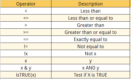
R Logical Operators
With logical operators, we want to return values inside the vector based on logical conditions. Following is a detailed list of logical operators of data types in R programming
The logical statements in R are wrapped inside the []. We can add as many conditional statements as we like but we need to include them in a parenthesis. We can follow this structure to create a conditional statement:
variable_name[(conditional_statement)]
With variable_name referring to the variable, we want to use for the statement. We create the logical statement i.e. variable_name > 0. Finally, we use the square bracket to finalize the logical statement. Below, an example of a logical statement.
Example 1
# Create a vector from 1 to 10
logical_vector <- c(1:10)
logical_vector>5
Output:
## [1]FALSE FALSE FALSE FALSE FALSE TRUE TRUE TRUE TRUE TRUE
In the output above, R reads each value and compares it to the statement logical_vector>5. If the value is strictly superior to five, then the condition is TRUE, otherwise FALSE. R returns a vector of TRUE and FALSE.
Example 2
In the example below, we want to extract the values that only meet the condition ‘is strictly superior to five’. For that, we can wrap the condition inside a square bracket precede by the vector containing the values.
# Print value strictly above 5
logical_vector[(logical_vector>5)]
Output:
## [1] 6 7 8 9 10
Example 3
# Print 5 and 6
logical_vector <- c(1:10)
logical_vector[(logical_vector>4) & (logical_vector<7)]
Output:
## [1] 5 6