
R Data Frame: How to Create, Append, Select & Subset
 Editorial Team
⚡ Smart Summary
R Data Frame stores columns of different types at equal length, which makes it the standard rectangular structure for analysis. Square brackets slice rows and columns, the dollar sign reaches a column, and subset() filters by condition.

What is a Data Frame?
A data frame is a list of vectors which are of equal length. A matrix contains only one type of data, while a data frame accepts different data types (numeric, character, factor, etc.).
That definition places the data frame between two neighbours you will meet constantly in R. A matrix is rectangular but single-typed, and a list is multi-typed but ragged. The data frame borrows one property from each.
| Structure | Column types | Element lengths | Typical use |
|---|---|---|---|
| Vector | One type only | Single sequence | One variable |
| Matrix | One type only | Rectangular | Numeric algebra |
| List | Any mix of types | May differ per element | Arbitrary collections |
| Data frame | Any mix of types | Every column equal length | Tabular analysis |
Because a data frame really is a list underneath, the accessors used on lists work here too, which is why the dollar sign appears again later in this tutorial.
How to Create a Data Frame
We can create a dataframe in R by passing the variables a, b, c and d into the data.frame() function. We can create the data frame and name the columns with names(), simply specifying the name of each variable.
data.frame(df, stringsAsFactors = TRUE)
Arguments:
- df: It can be a matrix to convert as a data frame or a collection of variables to join
- stringsAsFactors: Controls whether character vectors become factor columns. The factory-fresh default was TRUE in older releases and has been FALSE since R 4.0.0, so pass it explicitly when the behaviour matters
We can create a dataframe in R for our first data set by combining four variables of same length.
# Create a, b, c, d variables
a <- c(10,20,30,40)
b <- c('book', 'pen', 'textbook', 'pencil_case')
c <- c(TRUE,FALSE,TRUE,FALSE)
d <- c(2.5, 8, 10, 7)
# Join the variables to create a data frame
df <- data.frame(a,b,c,d)
df
Output:
##     a         b     c     d
## 1  10        book  TRUE   2.5
## 2  20         pen  FALSE  8.0
## 3  30    textbook  TRUE   10.0
## 4  40 pencil_case  FALSE  7.0
Each vector became a column, and the four values in each vector became the four rows. Note that the arguments were unnamed, so R derived the column headers from the variable names themselves.
We can see the column headers have the same name as the variables. We can change column name in R with the function names(). Check the R create dataframe example below:
# Name the data frame
names(df) <- c('ID', 'items', 'store', 'price')
df
Output:
##   ID       items store price
## 1 10        book  TRUE   2.5
## 2 20         pen FALSE   8.0
## 3 30    textbook  TRUE  10.0
## 4 40 pencil_case FALSE   7.0
Assigning to names() replaces every header at once, so the replacement vector must have exactly one entry per column. To rename a single column instead, index the names vector, as in names(df)[2] <- ‘product’.
# Print the structure
str(df)
Output:
## 'data.frame':    4 obs. of  4 variables:
##  $ ID   : num  10 20 30 40
##  $ items: Factor w/ 4 levels "book","pen","pencil_case",..: 1 2 4 3
##  $ store: logi  TRUE FALSE TRUE FALSE
##  $ price: num  2.5 8 10 7
Version note. The output above was produced on an R release older than 4.0.0, where data.frame() converted character vectors to factors by default, which is why items is reported as a Factor with four levels. The base R documentation records that this factory-fresh default changed to stringsAsFactors = FALSE for R 4.0.0. Running the same code on a current release leaves items as a plain character column, and str() prints chr instead. Add stringsAsFactors = TRUE to the data.frame() call to reproduce the printed output, or read the factor tutorial for when factors are actually wanted.
Slice Data Frame
With the frame built, the next task is pulling parts of it back out. Slicing is the base R way to do that, and it uses the same square brackets as vectors, only with two positions instead of one.
It is possible to SLICE values of a Data Frame. We select the rows and columns to return inside brackets preceded by the name of the data frame.
A data frame is composed of rows and columns, df[A, B]. A represents the rows and B the columns. We can slice either by specifying the rows and/or columns.
From picture 1 below, the left part represents the rows, and the right part is the columns. Note that the symbol : means to. For instance, 1:3 intends to select values from 1 to 3.
![R data frame slicing syntax df[A, B] with rows on the left of the comma and columns on the right](https://www.guru99.com/images/r_programming/032918_1452_RDataFrames1.png)
In the diagram below we display how to access different selections of the data frame:
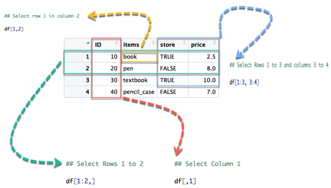
- The yellow arrow selects the row 1 in column 2
- The green arrow selects the rows 1 to 2
- The red arrow selects the column 1
- The blue arrow selects the rows 1 to 3 and columns 3 to 4
Note that, if we let the left part blank, R will select all the rows. By analogy, if we let the right part blank, R will select all the columns.
We can run the code in the console:
## Select row 1 in column 2
df[1,2]
Output:
## [1] book
## Levels: book pen pencil_case textbook
The Levels line appears because items is a factor in this session. On R 4.0.0 and later the same call prints the single string “book” with no Levels line.
## Select Rows 1 to 2
df[1:2,]
Output:
##   ID items store price
## 1 10  book  TRUE   2.5
## 2 20   pen FALSE   8.0
## Select Columns 1
df[,1]
Output:
## [1] 10 20 30 40
Selecting a single column with df[,1] drops the frame wrapper and returns a plain vector. Add drop = FALSE, as in df[, 1, drop = FALSE], when a one-column data frame is needed instead.
## Select Rows 1 to 3 and columns 3 to 4
df[1:3, 3:4]
Output:
##   store price
## 1  TRUE   2.5
## 2 FALSE   8.0
## 3  TRUE  10.0
It is also possible to select the columns with their names. For instance, the code below extracts two columns: ID and store.
# Slice with columns name
df[, c('ID', 'store')]
Output:
##   ID store
## 1 10  TRUE
## 2 20 FALSE
## 3 30  TRUE
## 4 40 FALSE
Names are safer than positions in production code, because inserting or reordering a column silently changes what df[, 3] refers to while df[, ‘store’] keeps pointing at the same data.
Append a Column to Data Frame
You can also append a column to a Data Frame. You need to use the symbol $ to name the new variable and add a column to a dataframe in R.
# Create a new vector
quantity <- c(10, 35, 40, 5)

# Add `quantity` to the `df` data frame
df$quantity <- quantity
df
Output:
##   ID       items store price quantity
## 1 10        book  TRUE   2.5       10
## 2 20         pen FALSE   8.0       35
## 3 30    textbook  TRUE  10.0       40
## 4 40 pencil_case FALSE   7.0        5
Note: The number of elements in the vector has to be equal to the number of elements in the data frame. Executing the following statement to add a column to the data frame in R
quantity <- c(10, 35, 40)
# Add `quantity` to the `df` data frame
df$quantity <- quantity
Gives error:
Error in `lt;-.data.frame`
(`*tmp*`, quantity, value = c(10, 35, 40))
replacement has 3 rows, data has 4
The message names the replacement operator for data frames and states both counts, so it tells you exactly what to fix. R only recycles a replacement when its length divides the row count evenly, which is why a length-1 value such as df$currency <- 'EUR' is accepted while a length-3 vector against four rows is refused. cbind() adds a column in the same way, and rbind() is its counterpart for adding rows.
Select a Column of a Data Frame
Sometimes, we need to store a column of a data frame for future use or perform an operation on a column. We can use the $ sign to select the column from a data frame.
# Select the column ID
df$ID
Output:
## [1] 1 2 3 4
Read that output with care. ID was built from the vector c(10, 20, 30, 40), so a live console prints 10 20 30 40 here; the 1 2 3 4 shown above are row positions rather than the stored values. The [1] at the start of the line is simply the index of the first element on that line, not part of the data.
Three routes reach the same column: df$ID, df[['ID']] and df[, 'ID']. The dollar sign performs partial matching, so df$I would still find ID, which is convenient at the console and risky in a saved script.
Subset a Data Frame
In the previous section, we selected an entire column without condition. It is possible to subset based on whether or not a certain condition was true.
We use the subset() function.
subset(x, condition)
arguments:
- x: data frame used to perform the subset
- condition: define the conditional statement
We want to return only the items with a price above 5, so we can do:
# Select price above 5
subset(df, subset = price > 5)
Output:
ID       items store price
2 20         pen FALSE     8
3 30    textbook  TRUE    10
4 40 pencil_case FALSE     7
The row labels 2, 3 and 4 are the original row names carried over from df, which is how you can tell that the first row was filtered out. subset() also accepts a select argument for choosing columns at the same time, and the equivalent bracket form is df[df$price > 5, ]. The bracket form keeps NA rows where the condition is missing, whereas subset() drops them, so the two are not always interchangeable.
