
Factor in R: Categorical Variable & Continuous Variables
 Editorial Team
⚡ Smart Summary
Factor in R stores categorical data as a vector of integer codes paired with a set of levels, which is how the language separates a limited group of categories from a continuous measurement.
What is Factor in R?
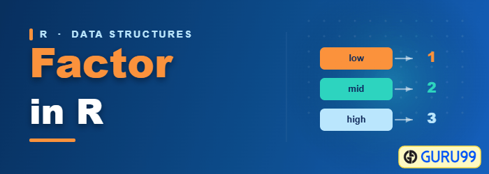
Factor in R is a variable used to categorize and store the data, having a limited number of different values. It stores the data as a vector of integer values. Factor in R is also known as a categorical variable that stores both string and integer data values as levels. Factor is mostly used in statistical modeling and exploratory data analysis with R.
Internally a factor is two objects travelling together: an integer vector of codes, and a character attribute named levels. Each code is a position in that levels vector, which is why printing a factor shows words while unclass() shows numbers.
In a dataset, we can distinguish two types of variables: categorical and continuous.
- In descriptive statistics for categorical variables in R, the value is limited and usually based on a particular finite group. For example, a categorical variable in R can be countries, year, gender, occupation.
- A continuous variable, however, can take any values, from integer to decimal. For example, we can have the revenue, price of a share, etc.
That distinction is worth guarding, because R silently chooses different defaults for each. A numeric column is summarised with a mean and a median, while a factor is summarised with counts per level. Storing a category as text or as a number therefore changes the analysis you get. The wider set of storage modes is covered in the guide to R data types and operators.
Categorical Variables
Categorical variables in R are stored into a factor. Let’s check the code below to convert a character variable into a factor variable in R. Many modelling and machine learning routines cannot consume raw text, so the categories have to be encoded as levels or as numbers before the model is fitted.
Syntax
factor(x = character(), levels, labels = levels, ordered = is.ordered(x))
The base R reference documents two further arguments that the shortened form above omits: exclude, which removes values before the level set is built, and nmax, an upper bound on the number of levels that speeds up conversion of very large vectors.
Arguments:
- x: A vector of categorical data in R. Needs to be a string or integer, not decimal.
- levels: A vector of possible values taken by x. This argument is optional. The default value is the unique list of items of the vector x, sorted into increasing order.
- labels: Add a label to the x categorical data in R. For example, 1 can take the label male while 0, the label female.
- exclude: A vector of values to drop when the level set is formed. Excluded values become NA in the result.
- ordered: A logical flag that determines whether the levels should be regarded as ordered, in the order given.
- nmax: An optional upper bound on the number of levels, useful for long vectors.
Example:
Let’s convert a character vector into a factor and confirm the change with class().
# Create gender vector
gender_vector <- c("Male", "Female", "Female", "Male", "Male")
class(gender_vector)
# Convert gender_vector to a factor
factor_gender_vector <-factor(gender_vector)
class(factor_gender_vector)
Output:
## [1] "character"
## [1] "factor"
The class switched from character to factor, and nothing about the printed values changed. It is important to transform a string into a factor variable in R before a machine learning task, because that is the point at which the categories become a fixed, validated set.
A categorical variable in R can be divided into nominal categorical variable and ordinal categorical variable.
Nominal Categorical Variable
A nominal categorical variable has several values but the order does not matter. For instance, male or female. Nominal categorical variables in R do not carry any ordering.
# Create a color vector
color_vector <- c('blue', 'red', 'green', 'white', 'black', 'yellow')
# Convert the vector to factor
factor_color <- factor(color_vector)
factor_color
Output:
## [1] blue   red    green  white  black  yellow
## Levels: black blue green red white yellow
From the factor_color, we can’t tell any order. The level list is alphabetical only because no levels argument was supplied, so R sorted the unique values itself. That sort follows the active locale rather than plain ASCII, which is one reason to state the levels explicitly whenever the order matters.
Ordinal Categorical Variable
Ordinal categorical variables do have a natural ordering. The ranking comes from the order of the vector passed to the levels argument, and ordered = TRUE tells R to treat that sequence as a ranking rather than a bare list. Setting ordered = FALSE does not reverse the ranking; it simply produces an ordinary unordered factor. To rank from highest to lowest, reverse the levels vector itself.
Example:
We can use summary to count the values for each factor variable in R.
# Create Ordinal categorical vector
day_vector <- c('evening', 'morning', 'afternoon', 'midday', 'midnight', 'evening')
# Convert `day_vector` to a factor with ordered level
factor_day <- factor(day_vector, order = TRUE, levels =c('morning', 'midday', 'afternoon', 'evening', 'midnight'))
# Print the new variable
factor_day
Output:
## [1] evening   morning   afternoon midday
midnight  evening
The console prints the values first and the ranking underneath. The next block opens with that Levels line, still commented out, so the ranking stays visible while the summary() call is appended to the previous code.
## Levels: morning < midday < afternoon < evening < midnight
# Append the line to above code
# Count the number of occurence of each level
summary(factor_day)
Output:
##   morning    midday afternoon   evening  midnight
##         1         1         1         2         1
R ordered the level from ‘morning’ to ‘midnight’ as specified in the levels argument. Because the factor is ordered, comparison operators such as < and > also work on it, which they do not on the nominal color factor above.
Continuous Variables
Continuous class variables are the default value in R. They are stored as numeric or integer. We can see it from the dataset below. mtcars is a built-in dataset. It gathers information on different types of cars. We can import it by using mtcars and check the class of the variable mpg, mile per gallon. It returns a numeric value, indicating a continuous variable.
dataset <- mtcars
class(dataset$mpg)
Output
## [1] "numeric"
Not every numeric column is genuinely continuous. In the same dataset, cyl holds only 4, 6 and 8, and am holds only 0 and 1, so both are categories that happen to be stored as numbers. Converting them with factor() before modelling stops R from treating the gap between 4 and 6 cylinders as a measured quantity. The reverse move, cutting a continuous column into bands, is handled by cut().
Factor Levels and Labels in R
The levels attribute is the part of a factor you will spend the most time adjusting, because it controls both what prints and what a model treats as the baseline. Four base R helpers cover almost every case.
| Function | What it does | Typical use |
|---|---|---|
| levels(f) | Reads or replaces the level names | Renaming abbreviations to readable labels |
| nlevels(f) | Returns the number of levels | Checking a category did not explode after a join |
| relevel(f, ref) | Moves one level to the front | Choosing the baseline for a regression |
| droplevels(f) | Removes levels with zero observations | Cleaning up after subsetting or filtering |
The block below applies all four to the color and gender factors created earlier.
# Inspect the levels of an existing factor
levels(factor_color)          # the level names, in the order R stored them
nlevels(factor_color)         # how many distinct levels exist

# Rename the levels in place (the new vector must follow the same order)
levels(factor_color) <- c('Black', 'Blue', 'Green', 'Red', 'White', 'Yellow')

# Attach labels at creation time instead of renaming afterwards
gender_coded <- factor(c(1, 0, 0, 1, 1), levels = c(0, 1), labels = c('female', 'male'))

# Make 'male' the reference level that modelling functions compare against
gender_coded <- relevel(gender_coded, ref = 'male')

# Remove levels that survived a subset but no longer occur in the data
subset_color <- droplevels(factor_color[1:3])
Two details are worth remembering. Assigning to levels() renames by position, so a mismatched vector silently relabels the wrong category. And a subset keeps every original level until droplevels() is called, which is why a filtered data frame can still plot empty bars. The labels argument is different again: it names the levels at creation time, and duplicated labels merge several input values into one level.
How to Convert a Factor to Numeric or Character in R
This is the single most common factor bug in R. Because a factor stores integer codes, calling as.numeric() on it returns those codes rather than the values you can see on screen. A factor of years 2021 to 2023 comes back as 1, 2 and 3.
# A factor whose labels happen to look like numbers
year_factor <- factor(c('2021', '2023', '2022', '2023'))

# WRONG: this returns the internal codes 1, 3, 2, 3 - not the years
as.numeric(year_factor)

# RIGHT: read the label through the levels attribute first
as.numeric(levels(year_factor))[year_factor]

# Equivalent and easier to remember, but slightly slower
as.numeric(as.character(year_factor))

# Back to plain text
as.character(year_factor)
The base R documentation recommends as.numeric(levels(f))[f] as the correct and slightly faster route, with as.numeric(as.character(f)) as the easier-to-read equivalent. Both read the label first and convert afterwards.
- Factor to character: as.character(f) returns the labels as plain text.
- Factor to integer codes: as.integer(f) or unclass(f) when the codes are what you actually want.
- Character to factor: factor(x) or the faster as.factor(x) shortcut.
- Numeric to factor: factor(x) for discrete codes, cut(x, breaks) for continuous values that need banding.
One safeguard applies to all of them. If a value in x does not appear in the levels vector, factor() sets that element to NA instead of raising an error, so a stray space or a capitalisation difference can quietly delete rows. Comparing unique values before and after the conversion, or sorting the data frame on the new column, exposes the problem quickly.
Factor vs Character vs Numeric in R: When to Use Each
Choosing the storage mode early saves a great deal of debugging later. The table compares the three modes a column of text or codes can take.
| Property | Factor | Character | Numeric |
|---|---|---|---|
| Stored as | Integer codes plus a levels attribute | Strings | Doubles or integers |
| Fixed set of values | Yes, defined by levels | No | No |
| Custom display order | Yes, through levels | Alphabetical only | Numerical only |
| Arithmetic | Not allowed | Not allowed | Allowed |
| Model contrasts | Built automatically | Coerced first | Treated as a measurement |
Use a factor when the values come from a known, closed list, when the display or ranking order matters, or when the column feeds a model or a plot legend. Use character for free text, identifiers and anything you will parse or join on, such as names, notes and codes that keep arriving with new values. Use numeric only when the distance between two values is meaningful.
The block below shows the quickest ways to check what you actually have.
# Ask R what each column of a data frame actually is
sapply(mtcars, class)

# Direct membership tests
is.factor(factor_day)
is.ordered(factor_day)

# unclass() exposes the integer codes hiding behind the labels
unclass(factor_color)
Two habits keep the choice honest. Run sapply(df, class) after every import, because a single stray character in a numeric column turns the whole column to text. And convert to a factor as late as possible, after the data is cleaned and joined, so that dplyr joins and filters still compare plain strings rather than mismatched level sets.
