
Matrix Function in R: Create, Print, add Column & Slice
 Editorial Team
⚡ Smart Summary
Matrix in R is a two-dimensional array that holds a single data type across m rows and n columns, built with matrix(), extended with cbind() and rbind(), and reached through square brackets.

Matrix Function in R
A matrix function in R is a 2-dimensional array that has m number of rows and n number of columns. In other words, matrix in R programming is a combination of two or more vectors with the same data type.
Underneath, a matrix is simply a vector carrying a dim attribute of length two. That is why every element must share one type: the moment a character value joins numbers, the whole matrix is coerced to character. R stores the values in a single column-wise run and uses dim to decide where each row ends, so the choice of data type applies to the whole object at once.
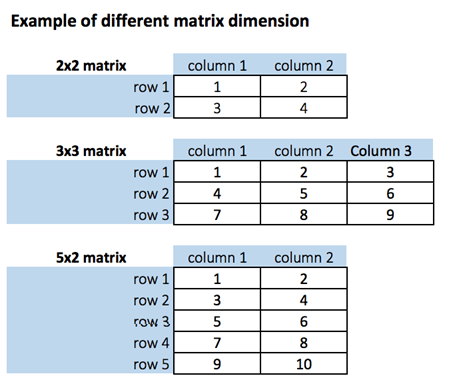
Note: matrix() itself always returns exactly two dimensions. To build a structure with three or more dimensions in R, use array() with a dim vector, or assign dim() directly. The diagram below shows the row and column layout that every matrix follows.
How to Create a Matrix in R
We can create a matrix with the function matrix(). The base R signature takes five arguments, and the three used most often are shown here:
matrix(data, nrow, ncol, byrow = FALSE)
Arguments:
- data: The collection of elements that R will arrange into the rows and columns of the matrix.
- nrow: Number of rows.
- ncol: Number of columns.
- byrow: A logical flag. With the default byrow = FALSE the matrix is filled column by column, top to bottom. With byrow = TRUE it is filled row by row, left to right.
- dimnames: An optional list of length two supplying the row names and the column names.
Two details from the base R reference are worth knowing before the first example. If only one of nrow and ncol is given, R infers the other from the length of data. And if data holds too few elements to fill the shape you asked for, the values are recycled rather than rejected.
Let’s construct two 5×2 matrices from the sequence of numbers 1 to 10, one with byrow = TRUE and one with byrow = FALSE, to see the difference.
# Construct a matrix with 5 rows that contain the numbers 1 up to 10 and byrow =  TRUE
matrix_a <-matrix(1:10, byrow = TRUE, nrow = 5)
matrix_a
Output:
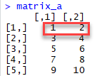
Because byrow = TRUE was used, the console fills the first row with 1 and 2, the second row with 3 and 4, and so on.
Print the dimension of matrix_a with dim()
Now, let’s print dimension of the matrix in R with dim(). The syntax to print matrix in R using dim() is:
# Print dimension of the matrix with dim()
dim(matrix_a)
Output:
## [1] 5 2
dim() returns the row count first and the column count second, confirming the 5×2 shape.
Fill a Matrix by Column with byrow = FALSE
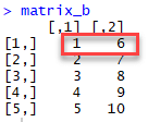
The same ten numbers and the same nrow produce a different arrangement once the filling direction changes. Keeping byrow at its default sends the values down the first column before the second one starts.
# Construct a matrix with 5 rows that contain the numbers 1 up to 10 and byrow =  FALSE
matrix_b <-matrix(1:10, byrow = FALSE, nrow = 5)
matrix_b
Output:
Print the dimension of matrix_b with dim()
Again, print the dimension of the matrix using dim(). Below is a syntax of R print matrix dimension:
# Print dimension of the matrix with dim()
dim(matrix_b)
Output:
## [1] 5 2
The shape is unchanged at 5×2, because byrow alters the filling order and never the dimensions.
Note: Using command matrix_b <-matrix(1:10, byrow = FALSE, ncol = 2) will have same effect as above, since R infers nrow = 5 from the ten values supplied.
You can also create a 4×3 matrix using ncol. R will create 3 columns and fill each column from top to bottom. Check an example
matrix_c <-matrix(1:12, byrow = FALSE, ncol = 3)
matrix_c
Output:
##       [,1] [,2] [,3]
## [1,]    1    5    9
## [2,]    2    6   10
## [3,]    3    7   11
## [4,]    4    8   12
The column headers [,1] to [,3] and the row labels [1,] to [4,] are R’s default placeholders. They disappear as soon as real dimnames are supplied, as shown later in this tutorial.
Example:
dim(matrix_c)
Output:
## [1] 4 3
Add a Column to a Matrix with the cbind()
You can add column to matrix R with the cbind() command. cbind() means column binding, and it can concatenate as many matrices or columns as specified. For example, our previous example created a 5×2 matrix. We concatenate a third column and verify the dimension is 5×3.
Example:
# concatenate c(1:5) to the matrix_a
matrix_a1 <- cbind(matrix_a, c(1:5))
# Check the dimension
dim(matrix_a1)
Output:
## [1] 5 3
Example:
matrix_a1
Output
##       [,1] [,2] [,3]
## [1,]    1    2    1
## [2,]    3    4    2
## [3,]    5    6    3
## [4,]    7    8    4
## [5,]    9   10    5
Example:
We can also bind more than one column at a time. The next block builds matrix_a2, a 4×3 matrix holding the numbers 13 to 24, so that it can be joined to the 4×3 matrix_c to produce a 4×6 result covering 1 to 24.
matrix_a2 <-matrix(13:24, byrow = FALSE, ncol = 3)
Output:
##      [,1] [,2] [,3]
## [1,]   13   17   21
## [2,]   14   18   22
## [3,]   15   19   23
## [4,]   16   20   24
Example:
matrix_c <-matrix(1:12, byrow = FALSE, ncol = 3)
matrix_d <- cbind(matrix_a2, matrix_c)
dim(matrix_d)
Output:
## [1] 4 6
NOTE: The number of rows of the matrices in R must be equal for cbind() to work. When they differ R either recycles the shorter input or raises an error, so checking dim() on both objects first is the safer habit.
Where cbind() concatenates columns, rbind() appends rows. Let’s add one row to our matrix_c matrix and verify the dimension is 5×3.
matrix_c <-matrix(1:12, byrow = FALSE, ncol = 3)
# Create a vector of 3 columns
add_row <- c(1:3)
# Append to the matrix
matrix_c <- rbind(matrix_c, add_row)
# Check the dimension
dim(matrix_c)
Output:
## [1] 5 3
Notice that binding a named vector such as add_row also gives the new row that name, which is the first step towards the labelled matrices covered further down.
Slice a Matrix
We can select one or many elements from a matrix in R programming by using the square brackets [ ]. Inside the brackets the row selector comes first and the column selector second, separated by a comma. This is where slicing comes into the picture.
For example:
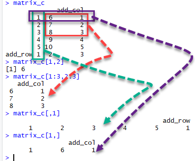
- matrix_c[1,2] selects the element at the first row and second column.
- matrix_c[1:3,2:3] results in a R slice matrix with the data on the rows 1, 2, 3 and columns 2 and 3.
- matrix_c[,1] selects all elements of the first column.
- matrix_c[1,] selects all elements of the first row.
Leaving a side of the comma blank therefore means every value on that side. One consequence catches beginners out: when a single row or column is selected, R drops the empty dimension and hands back a plain vector. Adding drop = FALSE, as in matrix_c[1, , drop = FALSE], keeps the result a matrix.
Here is the output you get for the above codes
Name the Rows and Columns of a Matrix in R
Default labels such as [,1] and [3,] make output hard to read as soon as a matrix carries real meaning. The dimnames argument, and the rownames() and colnames() replacement functions, attach text labels that then travel with the matrix through cbind(), t() and every slicing operation.
# Name the rows and columns while the matrix is built
sales <- matrix(1:6, nrow = 2, ncol = 3,
                dimnames = list(c('north', 'south'), c('q1', 'q2', 'q3')))

# Or attach the names afterwards
rownames(sales) <- c('north', 'south')
colnames(sales) <- c('q1', 'q2', 'q3')

# Read the names back as a list of two character vectors
dimnames(sales)

# Names make label based slicing possible
sales['north', 'q2']
| Function | Reads | Sets |
|---|---|---|
| dimnames(m) | Both dimensions as a list of two vectors | dimnames(m) <- list(rows, cols) |
| rownames(m) | The row labels | rownames(m) <- rows |
| colnames(m) | The column labels | colnames(m) <- cols |
| dim(m) | Rows and columns as two integers | dim(m) <- c(nrow, ncol) |
Once the labels exist, sales[‘north’, ‘q2’] is far clearer than sales[1, 2] and survives a reordering of the rows. Setting a dimnames component to NULL removes that set of labels again, and a matrix converted with as.data.frame() carries its row and column names straight into the data frame.
Matrix Operations in R: Arithmetic, Transpose and Multiplication
Arithmetic on matrices is where the single-type rule pays off. Base R handles the whole set without an extra package, but two operators are easy to confuse: * multiplies element by element, while %*% performs genuine matrix multiplication and requires the columns of the left operand to match the rows of the right one.
m1 <- matrix(1:4, nrow = 2)
m2 <- matrix(5:8, nrow = 2)

m1 + m2          # element by element addition
m1 * m2          # element by element product, NOT matrix multiplication
m1 %*% m2        # true matrix multiplication
t(m1)            # transpose: rows become columns
solve(m1)        # inverse, for a square matrix that is not singular

rowSums(m1)      # one total per row
colMeans(m1)     # one mean per column
apply(m1, 1, max)   # any function, applied row by row
- t(m): Transposes the matrix, so element [i, j] becomes [j, i]. Dimnames are carried across.
- solve(m): Returns the inverse of a square, non-singular matrix, and solve(a, b) solves a linear system.
- rowSums / colSums / rowMeans / colMeans: Documented as equivalent to apply() with sum or mean, but a great deal faster.
- apply(m, MARGIN, FUN): MARGIN = 1 walks the rows and MARGIN = 2 walks the columns, for any function you supply.
- diag, det, crossprod: Diagonal, determinant and the faster form of t(x) %*% y.
Because these operations are vectorised, they replace loops rather than sitting inside them. A summary that would take a nested for loop over thousands of cells becomes a single colMeans() call, which matters as soon as the data grows.
Matrix vs Data Frame vs Array in R
Matrices, data frames and arrays all look rectangular in the console, yet they answer different questions. The table sets them side by side.
| Property | Matrix | Data frame | Array |
|---|---|---|---|
| Dimensions | Exactly 2 | Exactly 2 | Any number |
| Column types | One type for the whole object | A different type per column | One type for the whole object |
| Built with | matrix() | data.frame() | array() |
| Typical use | Numeric computation and linear algebra | Mixed observational data | Stacked tables, such as counts by year |
| Row labels | Optional dimnames | Row names always present | Optional dimnames |
# A matrix holds one type only, so mixing coerces everything to character
mixed <- matrix(c(1, 2, 'a', 'b'), nrow = 2)
class(mixed[1, 1])

# Convert between the structures
as.data.frame(matrix_c)
as.matrix(mtcars)

# A matrix is the two dimensional case of an array
is.matrix(matrix_c)
inherits(matrix_c, 'array')
Reach for a matrix when every cell is the same kind of number and the work is arithmetic. Reach for a data frame when columns carry different types, for example a character name beside a numeric price and a factor. Reach for a list when the parts have different lengths, and for an array when a third index such as time or region genuinely exists. Conversion in either direction is cheap with as.matrix() and as.data.frame(), so the structure can follow the task rather than the other way round.
