Shortest Job First (SJF): Preemptive, Non-Preemptive Example

What is Shortest Job First Scheduling?

Shortest Job First (SJF) is an algorithm in which the process having the smallest execution time is chosen for the next execution. This scheduling method can be preemptive or non-preemptive. It significantly reduces the average waiting time for other processes awaiting execution. The full form of SJF is Shortest Job First.

There are basically two types of SJF methods:

• Non-Preemptive SJF
• Preemptive SJF

Characteristics of SJF Scheduling

• It is associated with each job as a unit of time to complete.
• This algorithm method is helpful for batch-type processing, where waiting for jobs to complete is not critical.
• It can improve process throughput by making sure that shorter jobs are executed first, hence possibly having a short turnaround time.
• It improves job output by offering shorter jobs, which should be executed first, and which mostly have a shorter turnaround time.

Non-Preemptive SJF

In non-preemptive scheduling, once the CPU cycle is allocated to a process, the process holds it till it reaches a waiting state or is terminated.

Consider the following five processes, each having its own unique burst time and arrival time.

Process Queue	Burst time	Arrival time
P1	6	2
P2	2	5
P3	8	1
P4	3	0
P5	4	4

Step 0) At time = 0, P4 arrives and starts execution.

Step 1) At time = 1, Process P3 arrives. But P4 still needs 2 execution units to complete. It will continue execution.

Step 2) At time = 2, process P1 arrives and is added to the waiting queue. P4 will continue execution.

Step 3) At time = 3, process P4 will finish its execution. The burst time of P3 and P1 is compared. Process P1 is executed because its burst time is less compared to P3.

Step 4) At time = 4, process P5 arrives and is added to the waiting queue. P1 will continue execution.

Step 5) At time = 5, process P2 arrives and is added to the waiting queue. P1 will continue execution.

Step 6) At time = 9, process P1 will finish its execution. The burst time of P3, P5, and P2 is compared. Process P2 is executed because its burst time is the lowest.

Step 7) At time = 10, P2 is executing and P3 and P5 are in the waiting queue.

Step 8) At time = 11, process P2 will finish its execution. The burst time of P3 and P5 is compared. Process P5 is executed because its burst time is lower.

Step 9) At time = 15, process P5 will finish its execution.

Step 10) At time = 23, process P3 will finish its execution.

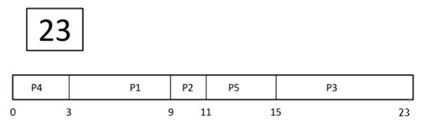
Step 11) Let us calculate the average waiting time for the above example.

Wait time
P4 = 0 - 0 = 0
P1 = 3 - 2 = 1
P2 = 9 - 5 = 4
P5 = 11 - 4 = 7
P3 = 15 - 1 = 14

Average Waiting Time = (0 + 1 + 4 + 7 + 14)/5 = 26/5 = 5.2

Preemptive SJF

In Preemptive SJF Scheduling, jobs are put into the ready queue as they come. A process with the shortest burst time begins execution. If a process with an even shorter burst time arrives, the current process is removed or preempted from execution, and the shorter job is allocated a CPU cycle.

Consider the following five processes:

Process Queue	Burst time	Arrival time
P1	6	2
P2	2	5
P3	8	1
P4	3	0
P5	4	4

Step 0) At time = 0, P4 arrives and starts execution.

Process Queue	Burst time	Arrival time
P1	6	2
P2	2	5
P3	8	1
P4	3	0
P5	4	4

Step 1) At time = 1, Process P3 arrives. But P4 has a shorter burst time. It will continue execution.

Step 2) At time = 2, process P1 arrives with burst time = 6. The burst time is more than that of P4. Hence, P4 will continue execution.

Step 3) At time = 3, process P4 will finish its execution. The burst time of P3 and P1 is compared. Process P1 is executed because its burst time is lower.

Step 4) At time = 4, process P5 will arrive. The burst time of P3, P5, and P1 is compared. Process P5 is executed because its burst time is lowest. Process P1 is preempted.

Process Queue	Burst time	Arrival time
P1	5 out of 6 is remaining	2
P2	2	5
P3	8	1
P4	3	0
P5	4	4

Step 5) At time = 5, process P2 will arrive. The burst time of P1, P2, P3, and P5 is compared. Process P2 is executed because its burst time is least. Process P5 is preempted.

Process Queue	Burst time	Arrival time
P1	5 out of 6 is remaining	2
P2	2	5
P3	8	1
P4	3	0
P5	3 out of 4 is remaining	4

Step 6) At time = 6, P2 is executing.

Step 7) At time = 7, P2 finishes its execution. The burst time of P1, P3, and P5 is compared. Process P5 is executed because its burst time is lesser.

Process Queue	Burst time	Arrival time
P1	5 out of 6 is remaining	2
P2	2	5
P3	8	1
P4	3	0
P5	3 out of 4 is remaining	4

Step 8) At time = 10, P5 will finish its execution. The burst time of P1 and P3 is compared. Process P1 is executed because its burst time is less.

Step 9) At time = 15, P1 finishes its execution. P3 is the only process left. It will start execution.

Step 10) At time = 23, P3 finishes its execution.

Step 11) Let us calculate the average waiting time for the above example.

Wait time
P4 = 0 - 0 = 0
P1 = (3 - 2) + 6 = 7
P2 = 5 - 5 = 0
P5 = 4 - 4 + 2 = 2
P3 = 15 - 1 = 14

Average Waiting Time = (0 + 7 + 0 + 2 + 14)/5 = 23/5 = 4.6

Advantages of SJF

Here are the benefits/pros of using the SJF method:

• SJF is frequently used for long term scheduling.
• It reduces the average waiting time over the FIFO (First In First Out) algorithm.
• The SJF method gives the lowest average waiting time for a specific set of processes.
• It is appropriate for the jobs running in batch, where run times are known in advance.
• For the batch system of long-term scheduling, a burst time estimate can be obtained from the job description.
• For Short-Term Scheduling, we need to predict the value of the next burst time.
• It is probably optimal with regard to average turnaround time.

Disadvantages/Cons of SJF

Here are some drawbacks/cons of the SJF algorithm:

• Job completion time must be known earlier, but it is hard to predict.
• It is often used in a batch system for long term scheduling.
• SJF cannot be implemented for CPU scheduling for the short term. It is because there is no specific method to predict the length of the upcoming CPU burst.
• This algorithm may cause very long turnaround times or starvation.
• Requires knowledge of how long a process or job will run.
• It leads to starvation that does not reduce average turnaround time.
• It is hard to know the length of the upcoming CPU request.
• Elapsed time should be recorded, which results in more overhead on the processor.

FAQs