
Scikit-Learn Tutorial: How to Install & Scikit-Learn Examples
 Editorial Team
⚡ Smart Summary
Scikit-learn is the open-source Python library that covers preprocessing, classification, regression, clustering and model selection behind a single consistent estimator interface, which keeps a complete machine learning workflow short, readable and reproducible from raw data to scored predictions.

What is Scikit-learn?
Scikit-learn is an open-source Python library for machine learning. It supports well-established algorithms such as KNN, gradient boosting, random forest and SVM, and it is built on top of NumPy and SciPy. Scikit-learn is widely used in Kaggle competitions as well as in prominent tech companies. It covers preprocessing, dimensionality reduction, classification, regression, clustering and model selection.
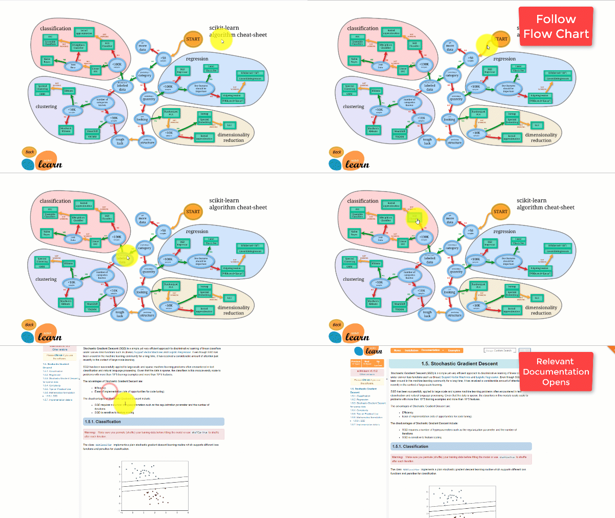
Scikit-learn has some of the best documentation of any open-source library. It even provides an interactive estimator chart, Choosing the right estimator, that walks you from the size of your dataset to a shortlist of algorithms worth trying.
The figure below illustrates how Scikit-learn works.
Scikit-learn is not difficult to use and gives excellent results. It does, however, train on the CPU: work is parallelised across cores with the n_jobs argument rather than on a GPU. Running a deep learning algorithm with it is possible but rarely optimal, especially if you already know how to use TensorFlow.
How to Download and Install Scikit-learn
Now in this Python Scikit-learn tutorial, you will learn how to download and install Scikit-learn:
Option 1: AWS
Scikit-learn can be used over AWS. A Docker image with scikit-learn preinstalled saves the setup work entirely.
To install the developer version, run the command below inside Jupyter:
import sys
!{sys.executable} -m pip install git+git://github.com/scikit-learn/scikit-learn.git
Option 2: Mac or Windows using Anaconda
To learn about Anaconda installation, refer to how to download and install TensorFlow.
At the time this walkthrough was written the developers of scikit had released a development version that fixed problems present in the then-current release, so the steps below use that developer build. On a fresh machine today the current stable release already contains every transformer used here, and pip install -U scikit-learn is enough.
How to Install scikit-learn with Conda Environment
If you installed scikit-learn with the conda environment, follow the steps below to update to version 0.20.
Step 1) Activate the tensorflow environment
source activate hello-tf
Step 2) Remove scikit-learn using the conda command
conda remove scikit-learn
Step 3) Install the developer version
Install the scikit-learn developer version along with the necessary libraries.
conda install -c anaconda git
pip install Cython
pip install h5py
pip install git+git://github.com/scikit-learn/scikit-learn.git
NOTE: Windows users need Microsoft Visual C++ 14. You can get it here.
Scikit-Learn Example with Machine Learning
This Scikit tutorial is divided into two parts:
- Machine learning with scikit-learn
- How to trust your model with LIME
The first part details how to build a pipeline, create a model and tune the hyperparameters, while the second part covers model interpretation.
Step 1) Import the data
During this Scikit learn tutorial, you will be using the adult census dataset.
The file is read straight from the UCI Machine Learning Repository in the code below, so no manual download is needed. If you are interested in the descriptive statistics, the Dive and Overview tools are worth a look. Refer to this tutorial to learn more about Dive and Overview.
You import the dataset with pandas. Note that you need to convert the continuous variables to float format.
This dataset includes eight categorical variables, listed in CATE_FEATURES:
- workclass
- education
- marital
- occupation
- relationship
- race
- sex
- native_country
It also includes six continuous variables, listed in CONTI_FEATURES:
- age
- fnlwgt
- education_num
- capital_gain
- capital_loss
- hours_week
The lists are filled by hand here so that you have a clearer idea of which columns are in play. A faster way to build a list of categorical or continuous columns is:
## List Categorical
CATE_FEATURES = df_train.iloc[:,:-1].select_dtypes('object').columns
print(CATE_FEATURES)

## List continuous
CONTI_FEATURES =  df_train._get_numeric_data()
print(CONTI_FEATURES)
Here is the code to import the data:
# Import dataset
import pandas as pd

## Define path data
COLUMNS = ['age','workclass', 'fnlwgt', 'education', 'education_num', 'marital',
           'occupation', 'relationship', 'race', 'sex', 'capital_gain', 'capital_loss',
           'hours_week', 'native_country', 'label']
### Define continuous list
CONTI_FEATURES  = ['age', 'fnlwgt','capital_gain', 'education_num', 'capital_loss', 'hours_week']
### Define categorical list
CATE_FEATURES = ['workclass', 'education', 'marital', 'occupation', 'relationship', 'race', 'sex', 'native_country']

## Prepare the data
features = ['age','workclass', 'fnlwgt', 'education', 'education_num', 'marital',
           'occupation', 'relationship', 'race', 'sex', 'capital_gain', 'capital_loss',
           'hours_week', 'native_country']

PATH = "https://archive.ics.uci.edu/ml/machine-learning-databases/adult/adult.data"

df_train = pd.read_csv(PATH, skipinitialspace=True, names = COLUMNS, index_col=False)
df_train[CONTI_FEATURES] =df_train[CONTI_FEATURES].astype('float64')
df_train.describe()
Calling describe() on the frame returns the summary statistics for the six continuous columns:
| age | fnlwgt | education_num | capital_gain | capital_loss | hours_week | |
|---|---|---|---|---|---|---|
| count | 32561.000000 | 3.256100e+04 | 32561.000000 | 32561.000000 | 32561.000000 | 32561.000000 |
| mean | 38.581647 | 1.897784e+05 | 10.080679 | 1077.648844 | 87.303830 | 40.437456 |
| std | 13.640433 | 1.055500e+05 | 2.572720 | 7385.292085 | 402.960219 | 12.347429 |
| min | 17.000000 | 1.228500e+04 | 1.000000 | 0.000000 | 0.000000 | 1.000000 |
| 25% | 28.000000 | 1.178270e+05 | 9.000000 | 0.000000 | 0.000000 | 40.000000 |
| 50% | 37.000000 | 1.783560e+05 | 10.000000 | 0.000000 | 0.000000 | 40.000000 |
| 75% | 48.000000 | 2.370510e+05 | 12.000000 | 0.000000 | 0.000000 | 45.000000 |
| max | 90.000000 | 1.484705e+06 | 16.000000 | 99999.000000 | 4356.000000 | 99.000000 |
You can check the count of unique values of the native_country feature. Only one household comes from Holand-Netherlands. That household brings no information and will throw an error during training.
df_train.native_country.value_counts()
United-States                 29170
Mexico                          643
?                               583
Philippines                     198
Germany                         137
Canada                          121
Puerto-Rico                     114
El-Salvador                     106
India                           100
Cuba                             95
England                          90
Jamaica                          81
South                            80
China                            75
Italy                            73
Dominican-Republic               70
Vietnam                          67
Guatemala                        64
Japan                            62
Poland                           60
Columbia                         59
Taiwan                           51
Haiti                            44
Iran                             43
Portugal                         37
Nicaragua                        34
Peru                             31
France                           29
Greece                           29
Ecuador                          28
Ireland                          24
Hong                             20
Cambodia                         19
Trinadad&Tobago                  19
Thailand                         18
Laos                             18
Yugoslavia                       16
Outlying-US(Guam-USVI-etc)       14
Honduras                         13
Hungary                          13
Scotland                         12
Holand-Netherlands                1
Name: native_country, dtype: int64
You can exclude this uninformative row from the dataset:
## Drop Netherland, because only one row
df_train = df_train[df_train.native_country != "Holand-Netherlands"]
Next, you store the position of the continuous features in a list. You will need it in the next step to build the pipeline.
The code below loops over all column names in CONTI_FEATURES, reads each location (that is, its column number) and appends it to a list called conti_features.
## Get the column index of the categorical features
conti_features = []
for i in CONTI_FEATURES:
    position = df_train.columns.get_loc(i)
    conti_features.append(position)
print(conti_features)
[0, 2, 10, 4, 11, 12]
The next block does the same job for the categorical variables.
## Get the column index of the categorical features
categorical_features = []
for i in CATE_FEATURES:
    position = df_train.columns.get_loc(i)
    categorical_features.append(position)
print(categorical_features)
[1, 3, 5, 6, 7, 8, 9, 13]
Now look at the dataset itself. Each categorical feature is a string, and a model cannot be fed a string value, so the dataset has to be transformed with dummy variables.
df_train.head(5)
In fact, you need one column for each group in each feature. First, run the code below to compute the total number of columns needed.
print(df_train[CATE_FEATURES].nunique(),
      'There are',sum(df_train[CATE_FEATURES].nunique()), 'groups in the whole dataset')
workclass          9
education         16
marital            7
occupation        15
relationship       6
race               5
sex                2
native_country    41
dtype: int64 There are 101 groups in the whole dataset
The whole dataset contains 101 groups, as shown above. The workclass feature alone has nine groups. You can list the names of the groups with the code below; unique() returns the distinct values of each categorical feature.
for i in CATE_FEATURES:
    print(df_train[i].unique())
['State-gov' 'Self-emp-not-inc' 'Private' 'Federal-gov' 'Local-gov' '?'
 'Self-emp-inc' 'Without-pay' 'Never-worked']
['Bachelors' 'HS-grad' '11th' 'Masters' '9th' 'Some-college' 'Assoc-acdm'
 'Assoc-voc' '7th-8th' 'Doctorate' 'Prof-school' '5th-6th' '10th'
 '1st-4th' 'Preschool' '12th']
['Never-married' 'Married-civ-spouse' 'Divorced' 'Married-spouse-absent'
 'Separated' 'Married-AF-spouse' 'Widowed']
['Adm-clerical' 'Exec-managerial' 'Handlers-cleaners' 'Prof-specialty'
 'Other-service' 'Sales' 'Craft-repair' 'Transport-moving'
 'Farming-fishing' 'Machine-op-inspct' 'Tech-support' '?'
 'Protective-serv' 'Armed-Forces' 'Priv-house-serv']
['Not-in-family' 'Husband' 'Wife' 'Own-child' 'Unmarried' 'Other-relative']
['White' 'Black' 'Asian-Pac-Islander' 'Amer-Indian-Eskimo' 'Other']
['Male' 'Female']
['United-States' 'Cuba' 'Jamaica' 'India' '?' 'Mexico' 'South'
 'Puerto-Rico' 'Honduras' 'England' 'Canada' 'Germany' 'Iran'
 'Philippines' 'Italy' 'Poland' 'Columbia' 'Cambodia' 'Thailand' 'Ecuador'
 'Laos' 'Taiwan' 'Haiti' 'Portugal' 'Dominican-Republic' 'El-Salvador'
 'France' 'Guatemala' 'China' 'Japan' 'Yugoslavia' 'Peru'
 'Outlying-US(Guam-USVI-etc)' 'Scotland' 'Trinadad&Tobago' 'Greece'
 'Nicaragua' 'Vietnam' 'Hong' 'Ireland' 'Hungary']
The training dataset will therefore contain 101 + 6 columns: the one-hot groups plus the six continuous features.
Scikit-learn can take care of the conversion, in two steps:
- Convert the string to an ID. State-gov becomes ID 1, Self-emp-not-inc becomes ID 2 and so on. LabelEncoder does this for you.
- Transpose each ID into a new column. The dataset has 101 group IDs, so there will be 101 columns capturing every categorical feature group. Scikit-learn provides OneHotEncoder for this operation.
Step 2) Create the train/test set
Now that the dataset is ready, split it 80/20: 80 percent for the training set and 20 percent for the test set.
You can use train_test_split. The first argument is the dataframe of features and the second is the label. You set the size of the test set with test_size.
from sklearn.model_selection import train_test_split
X_train, X_test, y_train, y_test = train_test_split(df_train[features],
                                                    df_train.label,
                                                    test_size = 0.2,
                                                    random_state=0)
X_train.head(5)
print(X_train.shape, X_test.shape)
(26048, 14) (6512, 14)
Step 3) Build the pipeline
The pipeline makes it easier to feed the model with consistent data. The idea is to push the raw data through one object that performs every operation in order.
With this dataset you need to standardise the continuous variables and convert the categorical ones. Any operation can live inside a pipeline: missing values can be replaced with the mean or median, and new variables can be created.
You have a choice: hard-code the two processes, or build a pipeline. Hard-coding can leak test data into the fitted statistics and creates inconsistencies over time, so the pipeline is the better option.
from sklearn.preprocessing import StandardScaler, OneHotEncoder, LabelEncoder
from sklearn.compose import ColumnTransformer, make_column_transformer
from sklearn.pipeline import make_pipeline
from sklearn.linear_model import LogisticRegression
The pipeline performs two operations before feeding the logistic classifier:
- Standardise the variable: StandardScaler()
- Convert the categorical features: OneHotEncoder(sparse=False)
You perform both steps with make_column_transformer. When this walkthrough was written the function was not in the released version of scikit-learn (0.19), which is why the developer build was used; it has shipped in every stable release since 0.20.
make_column_transformer is straightforward: you declare which columns to transform and which transformation to apply. To standardise the continuous features you pass:
- conti_features, StandardScaler() inside make_column_transformer
- conti_features: the list of continuous columns
- StandardScaler: standardises those columns
The OneHotEncoder object inside make_column_transformer encodes the labels automatically.
preprocess = make_column_transformer(
    (conti_features, StandardScaler()),
    ### Need to be numeric not string to specify columns name
    (categorical_features, OneHotEncoder(sparse=False))
)
Version note: two arguments in the block above have moved on. Current releases expect the transformer first and the columns second, and sparse was renamed sparse_output in scikit-learn 1.2 and removed in 1.4, so newer code reads OneHotEncoder(sparse_output=False).
You can test whether the pipeline works with fit_transform. The output should have the shape 26048, 107.
preprocess.fit_transform(X_train).shape
(26048, 107)
The data transformer is ready. You create the pipeline with make_pipeline, and once the data is transformed you feed the logistic regression.
model = make_pipeline(
    preprocess,
    LogisticRegression())
Training a model with scikit-learn is then trivial: call fit on the pipeline. You can print the accuracy with the score method.
model.fit(X_train, y_train)
print("logistic regression score: %f" % model.score(X_test, y_test))
logistic regression score: 0.850891
Finally, you can predict the classes with predict_proba, which returns the probability of each class. Note that the two probabilities sum to one.
model.predict_proba(X_test)
array([[0.83576663, 0.16423337],
       [0.94582765, 0.05417235],
       [0.64760587, 0.35239413],
       ...,
       [0.99639252, 0.00360748],
       [0.02072181, 0.97927819],
       [0.56781353, 0.43218647]])
Step 4) Using our pipeline in a grid search
Tuning the hyperparameters, the values that fix the structure of the model, can be tedious and exhausting.
One way to evaluate the model would be to change the size of the training set and measure the performance, repeating the exercise ten times to see the spread of the score. That is a lot of manual work.
Instead, scikit-learn provides functions that carry out parameter tuning and cross-validation for you.
Cross-validation
Cross-validation means that during training the training set is split n times into folds and the model is evaluated n times. If cv is set to 10, the model is trained and evaluated ten times. In each round the classifier trains on nine folds chosen at random and the tenth fold is kept for evaluation.
Grid search
Every classifier has hyperparameters to tune. You can try values one at a time, or set a parameter grid. The scikit-learn documentation lists all the parameters the logistic classifier accepts. To keep training fast, this example tunes only the C parameter, which controls regularisation. It must be positive, and a small value gives more weight to the regulariser.
You use the GridSearchCV object, which takes a dictionary of the hyperparameters to tune. List each hyperparameter followed by the values you want to try. To tune C you write:
- ‘logisticregression__C’: [0.001, 0.01, 0.1, 1.0] — the parameter name is preceded by the classifier name in lower case and two underscores.
The model will try four different values: 0.001, 0.01, 0.1 and 1. It is trained with 10 folds, that is cv=10.
from sklearn.model_selection import GridSearchCV
# Construct the parameter grid
param_grid = {
    'logisticregression__C': [0.001, 0.01,0.1, 1.0],
    }
You can now train the model using GridSearchCV with the parameter grid and cv.
# Train the model
grid_clf = GridSearchCV(model,
                        param_grid,
                        cv=10,
                        iid=False)
grid_clf.fit(X_train, y_train)
Output:
GridSearchCV(cv=10, error_score='raise-deprecating',
       estimator=Pipeline(memory=None,
     steps=[('columntransformer', ColumnTransformer(n_jobs=1, remainder='drop', transformer_weights=None,
         transformers=[('standardscaler', StandardScaler(copy=True, with_mean=True, with_std=True), [0, 2, 10, 4, 11, 12]), ('onehotencoder', OneHotEncoder(categorical_features=None, categories=None,...ty='l2', random_state=None, solver='liblinear', tol=0.0001,
          verbose=0, warm_start=False))]),
       fit_params=None, iid=False, n_jobs=1,
       param_grid={'logisticregression__C': [0.001, 0.01, 0.1, 1.0]},
       pre_dispatch='2*n_jobs', refit=True, return_train_score='warn',
       scoring=None, verbose=0)
Version note: the iid argument visible in this output was deprecated in scikit-learn 0.22 and removed in 0.24, so it should simply be dropped from the GridSearchCV call on current releases.
To access the best parameters, you use best_params_.
grid_clf.best_params_
Output:
{'logisticregression__C': 1.0}
After training the model with four different regularisation values, the optimal parameter gives:
print("best logistic regression from grid search: %f" % grid_clf.best_estimator_.score(X_test, y_test))
best logistic regression from grid search: 0.850891
To access the predicted probabilities:
grid_clf.best_estimator_.predict_proba(X_test)
array([[0.83576677, 0.16423323],
       [0.9458291 , 0.0541709 ],
       [0.64760416, 0.35239584],
       ...,
       [0.99639224, 0.00360776],
       [0.02072033, 0.97927967],
       [0.56782222, 0.43217778]])
XGBoost Model with scikit-learn
Now try one of the strongest classifiers on the market. XGBoost is a gradient-boosting improvement on the random forest. Its theoretical background is out of the scope of this Python Scikit tutorial, but keep in mind that XGBoost has won a great many Kaggle competitions. On an average-sized dataset it can perform as well as a deep learning algorithm, or better.
The classifier is challenging to train because it exposes a large number of parameters. You can of course use GridSearchCV to choose them for you.
A better option here is RandomizedSearchCV. GridSearchCV becomes slow when the grid is large, because the search space grows with every parameter added. RandomizedSearchCV instead samples the values of each hyperparameter at random on each iteration, so 1,000 iterations evaluate 1,000 combinations. It otherwise works much like GridSearchCV.
You need to import xgboost. If the library is not installed, run pip3 install xgboost, or install it from inside a Jupyter notebook with:
use import sys
!{sys.executable} -m pip install xgboost
Then import the classifier and the two search helpers:
import xgboost
from sklearn.model_selection import RandomizedSearchCV
from sklearn.model_selection import StratifiedKFold
The next step in this Scikit Python tutorial is to specify the parameters to tune. The official XGBoost documentation lists them all. For the sake of this Python Sklearn tutorial you choose only two hyperparameters with two values each, because XGBoost takes a long time to train and every extra grid point adds to the wait.
params = {
        'xgbclassifier__gamma': [0.5, 1],
        'xgbclassifier__max_depth': [3, 4]
        }
You then construct a new pipeline with the XGBoost classifier and 600 estimators. n_estimators is itself tunable, and a high value can lead to overfitting. You can try other values, but be aware that it can take hours. Every other parameter keeps its default.
model_xgb = make_pipeline(
    preprocess,
    xgboost.XGBClassifier(
                          n_estimators=600,
                          objective='binary:logistic',
                          silent=True,
                          nthread=1)
)
You can improve the cross-validation with the Stratified K-Folds cross-validator. Only three folds are used here to speed up the computation, at some cost in quality; increase this to 5 or 10 on your own machine for better results. The model is trained over four iterations.
skf = StratifiedKFold(n_splits=3,
                      shuffle = True,
                      random_state = 1001)

random_search = RandomizedSearchCV(model_xgb,
                                   param_distributions=params,
                                   n_iter=4,
                                   scoring='accuracy',
                                   n_jobs=4,
                                   cv=skf.split(X_train, y_train),
                                   verbose=3,
                                   random_state=1001)
The randomized search is ready, so you can train the model.
#grid_xgb = GridSearchCV(model_xgb, params, cv=10, iid=False)
random_search.fit(X_train, y_train)
Fitting 3 folds for each of 4 candidates, totalling 12 fits
[CV] xgbclassifier__max_depth=3, xgbclassifier__gamma=0.5 ............
[CV] xgbclassifier__max_depth=3, xgbclassifier__gamma=0.5 ............
[CV] xgbclassifier__max_depth=3, xgbclassifier__gamma=0.5 ............
[CV] xgbclassifier__max_depth=4, xgbclassifier__gamma=0.5 ............
[CV]  xgbclassifier__max_depth=3, xgbclassifier__gamma=0.5, score=0.8759645283888057, total= 1.0min
[CV] xgbclassifier__max_depth=4, xgbclassifier__gamma=0.5 ............
[CV]  xgbclassifier__max_depth=3, xgbclassifier__gamma=0.5, score=0.8729701715996775, total= 1.0min
[CV]  xgbclassifier__max_depth=3, xgbclassifier__gamma=0.5, score=0.8706519235199263, total= 1.0min
[CV] xgbclassifier__max_depth=4, xgbclassifier__gamma=0.5 ............
[CV] xgbclassifier__max_depth=3, xgbclassifier__gamma=1 ..............
[CV]  xgbclassifier__max_depth=4, xgbclassifier__gamma=0.5, score=0.8735460094437406, total= 1.3min
[CV] xgbclassifier__max_depth=3, xgbclassifier__gamma=1 ..............
[CV]  xgbclassifier__max_depth=3, xgbclassifier__gamma=1, score=0.8722791661868018, total=  57.7s
[CV] xgbclassifier__max_depth=3, xgbclassifier__gamma=1 ..............
[CV]  xgbclassifier__max_depth=3, xgbclassifier__gamma=1, score=0.8753886905447426, total= 1.0min
[CV] xgbclassifier__max_depth=4, xgbclassifier__gamma=1 ..............
[CV]  xgbclassifier__max_depth=4, xgbclassifier__gamma=0.5, score=0.8697304768486523, total= 1.3min
[CV] xgbclassifier__max_depth=4, xgbclassifier__gamma=1 ..............
[CV]  xgbclassifier__max_depth=4, xgbclassifier__gamma=0.5, score=0.8740066797189912, total= 1.4min
[CV] xgbclassifier__max_depth=4, xgbclassifier__gamma=1 ..............
[CV]  xgbclassifier__max_depth=3, xgbclassifier__gamma=1, score=0.8707671043538355, total= 1.0min
[CV]  xgbclassifier__max_depth=4, xgbclassifier__gamma=1, score=0.8729701715996775, total= 1.2min
[Parallel(n_jobs=4)]: Done  10 out of  12 | elapsed:  3.6min remaining:   43.5s
[CV]  xgbclassifier__max_depth=4, xgbclassifier__gamma=1, score=0.8736611770125533, total= 1.2min
[CV]  xgbclassifier__max_depth=4, xgbclassifier__gamma=1, score=0.8692697535130154, total= 1.2min
[Parallel(n_jobs=4)]: Done  12 out of  12 | elapsed:  3.6min finished
/Users/Thomas/anaconda3/envs/hello-tf/lib/python3.6/site-packages/sklearn/model_selection/_search.py:737: DeprecationWarning: The default of the `iid` parameter will change from True to False in version 0.22 and will be removed in 0.24. This will change numeric results when test-set sizes are unequal. DeprecationWarning)
RandomizedSearchCV(cv=<generator object _BaseKFold.split at 0x1101eb830>,
          error_score='raise-deprecating',
          estimator=Pipeline(memory=None,
     steps=[('columntransformer', ColumnTransformer(n_jobs=1, remainder='drop', transformer_weights=None,
         transformers=[('standardscaler', StandardScaler(copy=True, with_mean=True, with_std=True), [0, 2, 10, 4, 11, 12]), ('onehotencoder', OneHotEncoder(categorical_features=None, categories=None,...
       reg_alpha=0, reg_lambda=1, scale_pos_weight=1, seed=None,
       silent=True, subsample=1))]),
          fit_params=None, iid='warn', n_iter=4, n_jobs=4,
          param_distributions={'xgbclassifier__gamma': [0.5, 1], 'xgbclassifier__max_depth': [3, 4]},
          pre_dispatch='2*n_jobs', random_state=1001, refit=True,
          return_train_score='warn', scoring='accuracy', verbose=3)
As you can see, XGBoost scores better than the earlier logistic regression.
print("Best parameter", random_search.best_params_)
print("best logistic regression from grid search: %f" % random_search.best_estimator_.score(X_test, y_test))
Best parameter {'xgbclassifier__max_depth': 3, 'xgbclassifier__gamma': 0.5}
best logistic regression from grid search: 0.873157
random_search.best_estimator_.predict(X_test)
array(['<=50K', '<=50K', '<=50K', ..., '<=50K', '>50K', '<=50K'], dtype=object)
Create DNN with MLPClassifier in scikit-learn
Finally, you can train a neural network with scikit-learn itself. The method is the same as for any other classifier, and the estimator is MLPClassifier.
from sklearn.neural_network import MLPClassifier
The network below is defined with:
- Adam solver
- ReLU activation function
- Alpha = 0.0001
- Batch size of 150
- Two hidden layers with 200 and 100 neurons respectively
model_dnn = make_pipeline(
    preprocess,
    MLPClassifier(solver='adam',
                  alpha=0.0001,
                  activation='relu',
                    batch_size=150,
                    hidden_layer_sizes=(200, 100),
                    random_state=1))
You can change the number of layers to improve the model.
model_dnn.fit(X_train, y_train)
  print("DNN regression score: %f" % model_dnn.score(X_test, y_test))
DNN regression score: 0.821253
LIME: Trust your Model
Now that you have a good model, you need a way to trust it. Machine learning algorithms, especially random forests and neural networks, are known as black-box models: they work, but nobody can see why.
Three researchers built a tool that shows how the computer reaches a prediction. Their paper is “Why Should I Trust You?”, and the algorithm they published is called Local Interpretable Model-Agnostic Explanations (LIME).
Take an example. Sometimes you do not know whether a machine learning prediction can be trusted. A doctor cannot accept a diagnosis simply because a computer produced it, and you need to know whether a model is reliable before putting it into production.
Imagine being able to see why any classifier made a prediction, even for models as complicated as neural networks, random forests or SVMs with an arbitrary kernel. It becomes far easier to trust a prediction when the reasons behind it are visible, and equally easier to decide when a model should not be trusted. LIME tells you which features drove the decision of the classifier.
Data Preparation
There are a couple of things you need to change to run LIME with Python. First, install lime in the terminal with pip install lime.
Lime uses a LimeTabularExplainer object to approximate the model locally. This object requires:
- a dataset in NumPy format
- The name of the features: feature_names
- The name of the classes: class_names
- The index of the column of the categorical features: categorical_features
- The name of the group for each categorical feature: categorical_names
Create the NumPy train set
You can copy and convert df_train from pandas to NumPy very easily.
df_train.head(5)
# Create numpy data
df_lime = df_train
df_lime.head(3)
Get the class name
The label is accessible through unique(). You should see:
- ‘<=50K’
- ‘>50K’
# Get the class name
class_names = df_lime.label.unique()
class_names
array(['<=50K', '>50K'], dtype=object)
Index the categorical feature columns
Use the method you learned earlier to get the name of each group. You encode the label with LabelEncoder and repeat the operation on every categorical feature.
##
import sklearn.preprocessing as preprocessing
categorical_names = {}
for feature in CATE_FEATURES:
    le = preprocessing.LabelEncoder()
    le.fit(df_lime[feature])
    df_lime[feature] = le.transform(df_lime[feature])
    categorical_names[feature] = le.classes_
print(categorical_names)
{'workclass': array(['?', 'Federal-gov', 'Local-gov', 'Never-worked', 'Private',
       'Self-emp-inc', 'Self-emp-not-inc', 'State-gov', 'Without-pay'],
      dtype=object), 'education': array(['10th', '11th', '12th', '1st-4th', '5th-6th', '7th-8th', '9th',
       'Assoc-acdm', 'Assoc-voc', 'Bachelors', 'Doctorate', 'HS-grad',
       'Masters', 'Preschool', 'Prof-school', 'Some-college'],
      dtype=object), 'marital': array(['Divorced', 'Married-AF-spouse', 'Married-civ-spouse',
       'Married-spouse-absent', 'Never-married', 'Separated', 'Widowed'],
      dtype=object), 'occupation': array(['?', 'Adm-clerical', 'Armed-Forces', 'Craft-repair',
       'Exec-managerial', 'Farming-fishing', 'Handlers-cleaners',
       'Machine-op-inspct', 'Other-service', 'Priv-house-serv',
       'Prof-specialty', 'Protective-serv', 'Sales', 'Tech-support',
       'Transport-moving'], dtype=object), 'relationship': array(['Husband', 'Not-in-family', 'Other-relative', 'Own-child',
       'Unmarried', 'Wife'], dtype=object), 'race': array(['Amer-Indian-Eskimo', 'Asian-Pac-Islander', 'Black', 'Other',
       'White'], dtype=object), 'sex': array(['Female', 'Male'], dtype=object), 'native_country': array(['?', 'Cambodia', 'Canada', 'China', 'Columbia', 'Cuba',
       'Dominican-Republic', 'Ecuador', 'El-Salvador', 'England',
       'France', 'Germany', 'Greece', 'Guatemala', 'Haiti', 'Honduras',
       'Hong', 'Hungary', 'India', 'Iran', 'Ireland', 'Italy', 'Jamaica',
       'Japan', 'Laos', 'Mexico', 'Nicaragua',
       'Outlying-US(Guam-USVI-etc)', 'Peru', 'Philippines', 'Poland',
       'Portugal', 'Puerto-Rico', 'Scotland', 'South', 'Taiwan',
       'Thailand', 'Trinadad&Tobago', 'United-States', 'Vietnam',
       'Yugoslavia'], dtype=object)}

df_lime.dtypes
age               float64
workclass           int64
fnlwgt            float64
education           int64
education_num     float64
marital             int64
occupation          int64
relationship        int64
race                int64
sex                 int64
capital_gain      float64
capital_loss      float64
hours_week        float64
native_country      int64
label              object
dtype: object
Now that the dataset is ready, you can build the different datasets shown in the Scikit learn examples below. The data is transformed outside the pipeline here in order to avoid errors with LIME: the training set passed to LimeTabularExplainer must be a NumPy array with no strings, and the method above has already produced one.
from sklearn.model_selection import train_test_split
X_train_lime, X_test_lime, y_train_lime, y_test_lime = train_test_split(df_lime[features],
                                                    df_lime.label,
                                                    test_size = 0.2,
                                                    random_state=0)
X_train_lime.head(5)
You can make the pipeline with the optimal parameters found by XGBoost.
model_xgb = make_pipeline(
    preprocess,
    xgboost.XGBClassifier(max_depth = 3,
                          gamma = 0.5,
                          n_estimators=600,
                          objective='binary:logistic',
                          silent=True,
                          nthread=1))

model_xgb.fit(X_train_lime, y_train_lime)
/Users/Thomas/anaconda3/envs/hello-tf/lib/python3.6/site-packages/sklearn/preprocessing/_encoders.py:351: FutureWarning: The handling of integer data will change in version 0.22. Currently, the categories are determined based on the range [0, max(values)], while in the future they will be determined based on the unique values.
If you want the future behavior and silence this warning, you can specify "categories='auto'."In case you used a LabelEncoder before this OneHotEncoder to convert the categories to integers, then you can now use the OneHotEncoder directly.
  warnings.warn(msg, FutureWarning)
Pipeline(memory=None,
     steps=[('columntransformer', ColumnTransformer(n_jobs=1, remainder='drop', transformer_weights=None,
         transformers=[('standardscaler', StandardScaler(copy=True, with_mean=True, with_std=True), [0, 2, 10, 4, 11, 12]), ('onehotencoder', OneHotEncoder(categorical_features=None, categories=None,...
       reg_alpha=0, reg_lambda=1, scale_pos_weight=1, seed=None,
       silent=True, subsample=1))])
You get a warning. It explains that you do not need to create a label encoder before the pipeline. If you are not using LIME, the method from the first part of this Machine Learning with Scikit-learn tutorial is fine. Otherwise, keep this approach: first create an encoded dataset, then apply the one-hot encoder inside the pipeline.
print("best logistic regression from grid search: %f" % model_xgb.score(X_test_lime, y_test_lime))
best logistic regression from grid search: 0.873157
model_xgb.predict_proba(X_test_lime)
array([[7.9646105e-01, 2.0353897e-01],
       [9.5173013e-01, 4.8269872e-02],
       [7.9344827e-01, 2.0655173e-01],
       ...,
       [9.9031430e-01, 9.6856682e-03],
       [6.4581633e-04, 9.9935418e-01],
       [9.7104281e-01, 2.8957171e-02]], dtype=float32)
Before putting LIME to work, create a NumPy array holding the features of the wrongly classified rows. You can use that list later to get an idea of what misled the classifier.
temp = pd.concat([X_test_lime, y_test_lime], axis= 1)
temp['predicted'] = model_xgb.predict(X_test_lime)
temp['wrong']=  temp['label'] != temp['predicted']
temp = temp.query('wrong==True').drop('wrong', axis=1)
temp= temp.sort_values(by=['label'])
temp.shape
(826, 16)
You then create a lambda function that retrieves the prediction from the model for new data. You will need it shortly.
predict_fn = lambda x: model_xgb.predict_proba(x).astype(float)
X_test_lime.dtypes
age               float64
workclass           int64
fnlwgt            float64
education           int64
education_num     float64
marital             int64
occupation          int64
relationship        int64
race                int64
sex                 int64
capital_gain      float64
capital_loss      float64
hours_week        float64
native_country      int64
dtype: object
predict_fn(X_test_lime)
array([[7.96461046e-01, 2.03538969e-01],
       [9.51730132e-01, 4.82698716e-02],
       [7.93448269e-01, 2.06551731e-01],
       ...,
       [9.90314305e-01, 9.68566816e-03],
       [6.45816326e-04, 9.99354184e-01],
       [9.71042812e-01, 2.89571714e-02]])
You convert the pandas dataframe to a NumPy array.
X_train_lime = X_train_lime.values
X_test_lime = X_test_lime.values
X_test_lime
array([[4.00000e+01, 5.00000e+00, 1.93524e+05, ..., 0.00000e+00,
        4.00000e+01, 3.80000e+01],
       [2.70000e+01, 4.00000e+00, 2.16481e+05, ..., 0.00000e+00,
        4.00000e+01, 3.80000e+01],
       [2.50000e+01, 4.00000e+00, 2.56263e+05, ..., 0.00000e+00,
        4.00000e+01, 3.80000e+01],
       ...,
       [2.80000e+01, 6.00000e+00, 2.11032e+05, ..., 0.00000e+00,
        4.00000e+01, 2.50000e+01],
       [4.40000e+01, 4.00000e+00, 1.67005e+05, ..., 0.00000e+00,
        6.00000e+01, 3.80000e+01],
       [5.30000e+01, 4.00000e+00, 2.57940e+05, ..., 0.00000e+00,
        4.00000e+01, 3.80000e+01]])
model_xgb.predict_proba(X_test_lime)
array([[7.9646105e-01, 2.0353897e-01],
       [9.5173013e-01, 4.8269872e-02],
       [7.9344827e-01, 2.0655173e-01],
       ...,
       [9.9031430e-01, 9.6856682e-03],
       [6.4581633e-04, 9.9935418e-01],
       [9.7104281e-01, 2.8957171e-02]], dtype=float32)
print(features,
      class_names,
      categorical_features,
      categorical_names)
['age', 'workclass', 'fnlwgt', 'education', 'education_num', 'marital', 'occupation', 'relationship', 'race', 'sex', 'capital_gain', 'capital_loss', 'hours_week', 'native_country'] ['<=50K' '>50K'] [1, 3, 5, 6, 7, 8, 9, 13] {'workclass': array(['?', 'Federal-gov', 'Local-gov', 'Never-worked', 'Private',
       'Self-emp-inc', 'Self-emp-not-inc', 'State-gov', 'Without-pay'],
      dtype=object), 'education': array(['10th', '11th', '12th', '1st-4th', '5th-6th', '7th-8th', '9th',
       'Assoc-acdm', 'Assoc-voc', 'Bachelors', 'Doctorate', 'HS-grad',
       'Masters', 'Preschool', 'Prof-school', 'Some-college'],
      dtype=object), 'marital': array(['Divorced', 'Married-AF-spouse', 'Married-civ-spouse',
       'Married-spouse-absent', 'Never-married', 'Separated', 'Widowed'],
      dtype=object), 'occupation': array(['?', 'Adm-clerical', 'Armed-Forces', 'Craft-repair',
       'Exec-managerial', 'Farming-fishing', 'Handlers-cleaners',
       'Machine-op-inspct', 'Other-service', 'Priv-house-serv',
       'Prof-specialty', 'Protective-serv', 'Sales', 'Tech-support',
       'Transport-moving'], dtype=object), 'relationship': array(['Husband', 'Not-in-family', 'Other-relative', 'Own-child',
       'Unmarried', 'Wife'], dtype=object), 'race': array(['Amer-Indian-Eskimo', 'Asian-Pac-Islander', 'Black', 'Other',
       'White'], dtype=object), 'sex': array(['Female', 'Male'], dtype=object), 'native_country': array(['?', 'Cambodia', 'Canada', 'China', 'Columbia', 'Cuba',
       'Dominican-Republic', 'Ecuador', 'El-Salvador', 'England',
       'France', 'Germany', 'Greece', 'Guatemala', 'Haiti', 'Honduras',
       'Hong', 'Hungary', 'India', 'Iran', 'Ireland', 'Italy', 'Jamaica',
       'Japan', 'Laos', 'Mexico', 'Nicaragua',
       'Outlying-US(Guam-USVI-etc)', 'Peru', 'Philippines', 'Poland',
       'Portugal', 'Puerto-Rico', 'Scotland', 'South', 'Taiwan',
       'Thailand', 'Trinadad&Tobago', 'United-States', 'Vietnam',
       'Yugoslavia'], dtype=object)}
import lime
import lime.lime_tabular
### Train should be label encoded not one hot encoded
explainer = lime.lime_tabular.LimeTabularExplainer(X_train_lime ,
                                                   feature_names = features,
                                                   class_names=class_names,
                                                   categorical_features=categorical_features,
                                                   categorical_names=categorical_names,
                                                   kernel_width=3)
Now choose a random household from the test set and see both the prediction and how the computer arrived at it.
import numpy as np
np.random.seed(1)
i = 100
print(y_test_lime.iloc[i])
>50K
X_test_lime[i]
array([4.20000e+01, 4.00000e+00, 1.76286e+05, 7.00000e+00, 1.20000e+01,
       2.00000e+00, 4.00000e+00, 0.00000e+00, 4.00000e+00, 1.00000e+00,
       0.00000e+00, 0.00000e+00, 4.00000e+01, 3.80000e+01])
You can use the explainer with explain_instance to inspect the reasoning behind the model. The chart it renders is shown below.
exp = explainer.explain_instance(X_test_lime[i], predict_fn, num_features=6)
exp.show_in_notebook(show_all=False)

The classifier predicted this household correctly: the income is indeed above 50k.
The first thing to note is that the classifier is not very sure of itself. It predicts an income over 50k with a probability of 64%, and that 64% is driven by capital gain and marital status. The blue colour contributes negatively to the positive class and the orange line positively.
The classifier is hesitant because the capital gain of this household is zero, while capital gain is usually a good predictor of wealth. The household also works fewer than 40 hours per week. Age, occupation and sex all contribute positively.
If the marital status were single, the classifier would have predicted an income below 50k (0.64 – 0.18 = 0.46).
Now try another household, one that was classified wrongly. The explanation chart for it follows the code.
temp.head(3)
temp.iloc[1,:-2]
age                  58
workclass             4
fnlwgt            68624
education            11
education_num         9
marital               2
occupation            4
relationship          0
race                  4
sex                   1
capital_gain          0
capital_loss          0
hours_week           45
native_country       38
Name: 20931, dtype: object
i = 1
print('This observation is', temp.iloc[i,-2:])
This observation is label        <=50K
predicted     >50K
Name: 20931, dtype: object
exp = explainer.explain_instance(temp.iloc[1,:-2], predict_fn, num_features=6)
exp.show_in_notebook(show_all=False)

The classifier predicted an income below 50k, which is wrong. This household is unusual: it has neither a capital gain nor a capital loss, the person is divorced, close to 60 years old, and educated, that is education_num > 12. Following the overall pattern, the classifier placed the household below 50k.
Play with LIME yourself and you will notice plenty of blunt mistakes from the classifier. The GitHub repository of the library author carries extra documentation for image and text classification.
Scikit-learn Command Reference
Below is a list of useful commands that apply to scikit-learn version 0.20 and later.
| Task | Function or class |
|---|---|
| Create the train/test dataset | train_test_split |
| Build a pipeline | |
| Select the columns and apply the transformation | make_column_transformer |
| Type of transformation | |
| Standardise | StandardScaler |
| Min-max scaling | MinMaxScaler |
| Normalise | Normalizer |
| Impute missing values | SimpleImputer |
| Convert categorical | OneHotEncoder |
| Fit and transform the data | fit_transform |
| Make the pipeline | make_pipeline |
| Basic model | |
| Logistic regression | LogisticRegression |
| XGBoost | XGBClassifier |
| Neural net | MLPClassifier |
| Grid search | GridSearchCV |
| Randomized search | RandomizedSearchCV |
