Greedy Algorithm with Example: What is, Method and Approach

What is a Greedy Algorithm?

A Greedy Algorithm recursively divides a set of resources based on the maximum immediate availability of that resource at any stage of execution.

Solving a problem with the greedy approach has two stages:

1. Scanning the list of items
2. Optimization

Both stages run in parallel as the input array is progressively divided.

To follow the greedy approach, a working knowledge of recursion and context switching helps you trace the code. The greedy paradigm can be described with a pair of necessary and sufficient statements.

Two conditions define the greedy paradigm.

• Each stepwise choice must steer the problem toward its best-accepted solution.
• The problem structure must halt in a finite number of greedy steps.

With the theory in place, let us look at the history behind the greedy search approach.

History of Greedy Algorithms

Here are the important landmarks in the history of greedy algorithms:

• Greedy algorithms were first conceptualised for graph walk algorithms in the 1950s.
• Edsger Dijkstra developed his shortest-path algorithm to shorten routes across the Dutch capital, Amsterdam.
• In the same decade, Prim and Kruskal developed optimisation strategies that minimise path costs along weighted routes to build minimum spanning trees.
• In the ’70s, American researchers Cormen, Leiserson, Rivest, and Stein described recursive substructuring of greedy solutions in their classic Introduction to Algorithms textbook.
• The greedy search paradigm was catalogued as a distinct optimisation strategy in the NIST records in 2005.
• To this day, web protocols such as Open Shortest Path First (OSPF) and many packet-switching protocols use the greedy strategy to minimise transit time on a network.

Greedy Strategies and Decisions

The logic reduces to a binary choice at each stage — “greedy” or “not greedy” — based on the direction the algorithm takes to advance.

For example, Dijkstra’s algorithm identifies hosts on the Internet by evaluating a cost function at every step. The value the cost function returns decides whether the next path is “greedy” or “non-greedy”.

In short, an algorithm stops being greedy the moment it takes a step that is not locally optimal, and greedy problems halt when no further greedy step is possible.

Characteristics of the Greedy Algorithm

The important characteristics of a Greedy algorithm are:

• An ordered list of resources carries cost or value attributions that quantify the constraints on the system.
• The algorithm takes the maximum quantity of resources within the time a constraint applies.
• For example, in an activity scheduling problem the resource costs are measured in hours and the activities must be performed in serial order.

Why Use the Greedy Approach?

Here are the reasons for using the greedy approach:

• The greedy approach has trade-offs that make it well suited to optimisation.
• The most obvious reason is to produce a feasible solution immediately. In the activity selection problem discussed below, if more activities fit before the current activity finishes, they can be scheduled in the same window.
• Another reason is that it divides a problem recursively based on a condition, with no need to merge sub-solutions.
• In the activity selection problem, the recursive division step is achieved by scanning the list once and considering only the eligible activities.

How to Solve the Activity Selection Problem

In the activity scheduling example, every activity has a start and finish time and is indexed by a number for reference. There are two activity categories:

1. Considered activity: the reference activity from which the ability to fit more remaining activities is measured.
2. Remaining activities: activities at one or more indexes ahead of the considered activity.

The cost of performing an activity is its duration, calculated as (finish – start).

The greedy extent is simply the number of remaining activities that can be performed within the time of a considered activity.

Architecture of the Greedy Approach

Step 1) Scan the list of activity costs starting with index 0 as the considered index.

Step 2) When more activities can finish by the time the considered activity ends, search for those remaining activities.

Step 3) If no more activities can be scheduled, the current remaining activity becomes the next considered activity. Repeat Step 1 and Step 2 with the new considered activity. If no activities remain, go to Step 4.

Step 4) Return the union of considered indices — these are the activity indices that maximise throughput.

Architecture of the Greedy Approach

Code Explanation

#include<iostream>
#include<stdio.h>
#include<stdlib.h>

#define MAX_ACTIVITIES 12

Explanation of code:

1. Included header files/classes
2. The maximum number of activities configurable by the user.

using namespace std;

class TIME
{
    public:
    int hours;

    public: TIME()
    {
   	 hours = 0;
    }
};

Explanation of code:

1. Declares the standard namespace for streaming operations.
2. A class definition for TIME
3. An hour timestamp.
4. A TIME default constructor
5. The hours variable.

class Activity
{
    public:
    int index;
    TIME start;
    TIME finish;

    public: Activity()
    {
   	 start = finish = TIME();
    }
};

Explanation of code:

1. A class definition for Activity.
2. Timestamps that together define a duration.
3. All timestamps are initialised to 0 in the default constructor.

class Scheduler
{
    public:
    int considered_index,init_index;
    Activity *current_activities = new    Activity[MAX_ACTIVITIES];
    Activity *scheduled;

Explanation of code:

1. Part 1 of the scheduler class definition.
2. considered_index is the starting point for scanning the array.
3. init_index is used to assign random timestamps during setup.
4. An array of Activity objects is dynamically allocated with the new operator.
5. The scheduled pointer holds the current greedy result.

Scheduler()
{
   	 considered_index = 0;
   	 scheduled = NULL;
...
...

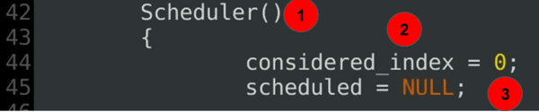
Explanation of code:

1. The Scheduler constructor — part 2 of the class definition.
2. considered_index marks the start of the current scan.
3. The greedy extent is undefined at the start.

for(init_index = 0; init_index < MAX_ACTIVITIES; init_index++)
 {
   		 current_activities[init_index].start.hours =
   			 rand() % 12;

   		 current_activities[init_index].finish.hours =
   			 current_activities[init_index].start.hours +
   				 (rand() % 2);

   		 printf("\nSTART:%d END %d\n",
   		 current_activities[init_index].start.hours
   		 ,current_activities[init_index].finish.hours);
 }
&#8230;
&#8230;

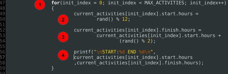
Explanation of code:

1. A for loop initialises the start and end hours of every scheduled activity.
2. Initialises the start time.
3. Initialises the end time to be at or after the start hour.
4. A debug statement prints the allocated durations.

	public:
   		 Activity * activity_select(int);
};

Explanation of code:

1. Part 4 — the final part of the Scheduler class definition.
2. activity_select() takes a starting index as the base and divides the greedy quest into subproblems.

Activity * Scheduler :: activity_select(int considered_index)
{
    this->considered_index = considered_index;
    int greedy_extent = this->considered_index + 1;
…
…

1. The scope resolution operator (::) links the function definition to the Scheduler class.
2. considered_index is passed by value, and greedy_extent is initialised to the index immediately after it.

Activity * Scheduler :: activity_select(int considered_index)
{
    	while( (greedy_extent < MAX_ACTIVITIES ) &&
   	 ((this->current_activities[greedy_extent]).start.hours <
   		 (this->current_activities[considered_index]).finish.hours ))
    	{
   	 printf("\nSchedule start:%d \nfinish%d\n activity:%d\n",
   	 (this->current_activities[greedy_extent]).start.hours,
   	 (this->current_activities[greedy_extent]).finish.hours,
   	 greedy_extent + 1);
   	 greedy_extent++;
    	}
&#8230;
...

Explanation of code:

1. The core logic — the greedy extent is capped at MAX_ACTIVITIES.
2. The start hour of the current activity is checked against the finish hour of the considered activity.
3. While the condition holds, an optional debug statement is printed.
4. The greedy extent then advances to the next index in the activity array.

...
if ( greedy_extent <= MAX_ACTIVITIES )
    {

   	 return activity_select(greedy_extent);
    }
    else
    {
   	 return NULL;
    }
}

Explanation of code:

1. The conditional checks whether all activities have been covered.
2. If not, the algorithm restarts the greedy quest from the current index — a recursive step that divides the problem greedily.
3. If yes, control returns to the caller with no scope for extending greed.

int main()
{
    Scheduler *activity_sched = new Scheduler();
    activity_sched->scheduled = activity_sched->activity_select(
   				activity_sched->considered_index);
    return 0;
}

Explanation of code:

1. The main function invokes the Scheduler.
2. A new Scheduler object is instantiated.
3. The activity_select() function returns an Activity pointer to the caller once the greedy quest ends.

Output:

START:7 END 7

START:9 END 10

START:5 END 6

START:10 END 10

START:9 END 10

Schedule start:5
finish6
 activity:3

Schedule start:9
finish10
 activity:5

Limitations of Greedy Technique

The greedy approach is not suitable for problems that require an optimal solution for every subproblem, such as sorting.

In such cases the greedy method can be wrong — in the worst case it produces a non-optimal solution.

The core drawback of greedy algorithms is that they choose without knowing what lies ahead of the current greedy state.

The diagram below illustrates this disadvantage of the greedy method.

In the greedy scan shown here as a tree (higher value means higher greed), an algorithm at value 40 would pick 29 next, then end at 12, for a total of 41.

By contrast, a divide-and-conquer strategy would follow 25 with 40 for a total of 65, which is 24 points higher than the locally greedy choice.

Examples of Greedy Algorithms

Most networking algorithms rely on a greedy approach. Common greedy algorithm examples include:

• Prim’s Minimum Spanning Tree Algorithm
• Travelling Salesman Problem (approximate)
• Graph Map Colouring
• Kruskal’s Minimum Spanning Tree Algorithm
• Dijkstra’s Shortest Path Algorithm
• Graph Vertex Cover
• Knapsack Problem
• Job Sequencing with Deadlines

FAQs