0/1 Knapsack Problem Fix using Dynamic Programming Example

What is the Knapsack Problem?

The Knapsack Problem is a classic combinatorial optimization problem. A supermarket stores n packages (n ≤ 100). Package i has weight W[i] ≤ 100 and value V[i] ≤ 100. A thief cannot carry weight exceeding capacity M (M ≤ 100). Which packages should the thief take to maximize total value?

Input:

• Maximum weight M and the number of packages n.
• Array of weight W[i] and corresponding value V[i].

Output:

• Maximum total value obtainable within the capacity.
• The exact set of packages the thief should take.

The Knapsack algorithm splits into two well-known variants:

• 0/1 Knapsack Problem solved by Dynamic Programming. Each package is either taken whole or left behind — no fractional pieces and no duplicates.
• Fractional Knapsack Problem solved by a Greedy Strategy. Here you may take a fraction of any package to fill the remaining capacity.

How to Solve Knapsack Problem using Dynamic Programming with Example

Divide-and-conquer splits a big problem into subproblems, then keeps splitting until each subproblem is easy. Plain recursion, however, often solves the same subproblem many times and wastes work.

The core idea of Knapsack Dynamic Programming is to store every solved subproblem in a table. Repeat calls read the answer instead of recomputing it, turning an exponential recursion into polynomial-time code.

Solve Knapsack Problem using Dynamic Programming

To design a Dynamic Programming solution, you follow four steps:

• Solve the smallest subproblems first.
• Derive a recurrence that builds a subproblem answer from smaller ones.
• Store subproblem answers in a table computed bottom-up using the recurrence.
• Assemble the final answer from the fully populated table.

Analyze the 0/1 Knapsack Problem

The optimal value depends on two independent factors:

1. How many packages are still being considered.
2. The remaining weight the knapsack can still store.

Because the objective function depends on two quantities, the table of options must be two-dimensional. Let B[i][j] denote the maximum value when choosing among packages {1, …, i} with weight limit j.

• The final answer is B[n][M], the best total value across all n packages under capacity M.
• The total selected weight is always bounded by the current capacity: B[i][j] ≤ j.

Example: if B[4][10] = 8, the best total weight from the first four packages under capacity 10 is 8. Some of those four packages may be skipped.

Formula to Calculate B[i][j]

• W[i], V[i] are the weight and value of package i, where i is in {1, …, n}.
• M is the maximum weight the knapsack can carry.

Base case with one package: for every capacity j ≥ W[1]:

B[1][j] = W[1]

For the general case, decide whether to include package i under capacity j:

• If package i is skipped, B[i][j] equals the best value using packages {1, …, i-1} under capacity j:

B[i][j] = B[i - 1][j]

• If package i is taken (allowed only when W[i] ≤ j), B[i][j] equals V[i] plus the best value from packages {1, …, i-1} under capacity j – W[i]:

B[i][j] = V[i] + B[i - 1][j - W[i]]

Take the larger of the two candidates.

Basis of Dynamic Programming

Combining the two cases gives the full recurrence:

B[i][j] = max(B[i - 1][j], V[i] + B[i - 1][j - W[i]])

The base case is B[0][j] = 0 for every j, because zero packages give zero value regardless of capacity.

Calculate the Table of Options

Build B using the recurrence. Once B is filled, the same table drives the trace-back that reconstructs the chosen packages. Table B has n + 1 rows and M + 1 columns:

• Row 0 is the base case, filled with zeros.
• Use row 0 to compute row 1, row 1 to compute row 2, and continue until row n is complete.

Table of Options

Trace

Once B is complete, focus on B[n][M], the optimal total value across all n packages with capacity M.

• If B[n][M] = B[n-1][M], package n was not selected, so continue tracing from B[n-1][M].
• If B[n][M] ≠ B[n-1][M], package n was selected, so continue tracing from B[n-1][M – W[n]].

Repeat until you reach row 0 of the table.

Algorithm to Look Up the Table of Options to Find the Selected Packages

Note: whenever B[i][j] = B[i-1][j], package i is not selected. The value B[n][M] is the optimal total value packed into the knapsack.

Steps for tracing the chosen packages:

• Step 1: Start at i = n, j = M.
• Step 2: Scan column j from bottom up until you find a row i where B[i][j] > B[i-1][j]. Mark package i as selected: Select[i] = true.
• Step 3: Update j = j – W[i]. If j > 0, return to Step 2, otherwise go to Step 4.
• Step 4: Print every package marked selected.

Java Code

The following Java method fills B[][] bottom-up, prints the table for inspection, and then traces the selected packages.

public void knapsackDyProg(int W[], int V[], int M, int n) {
    int B[][] = new int[n + 1][M + 1];

    for (int i = 0; i <= n; i++)
        for (int j = 0; j <= M; j++) {
            B[i][j] = 0;
        }

    for (int i = 1; i <= n; i++) {
        for (int j = 0; j <= M; j++) {
            B[i][j] = B[i - 1][j];

            if ((j >= W[i - 1]) && (B[i][j] < B[i - 1][j - W[i - 1]] + V[i - 1])) {
                B[i][j] = B[i - 1][j - W[i - 1]] + V[i - 1];
            }

            System.out.print(B[i][j] + " ");
        }
        System.out.print("\n");
    }

    System.out.println("Max Value:\t" + B[n][M]);
    System.out.println("Selected Packs: ");

    int j = M;
    while (n != 0) {
        if (B[n][j] != B[n - 1][j]) {
            System.out.println("\tPackage " + n + " with W = " + W[n - 1] + " and Value = " + V[n - 1]);
            j = j - W[n - 1];
        }
        n--;
    }
}

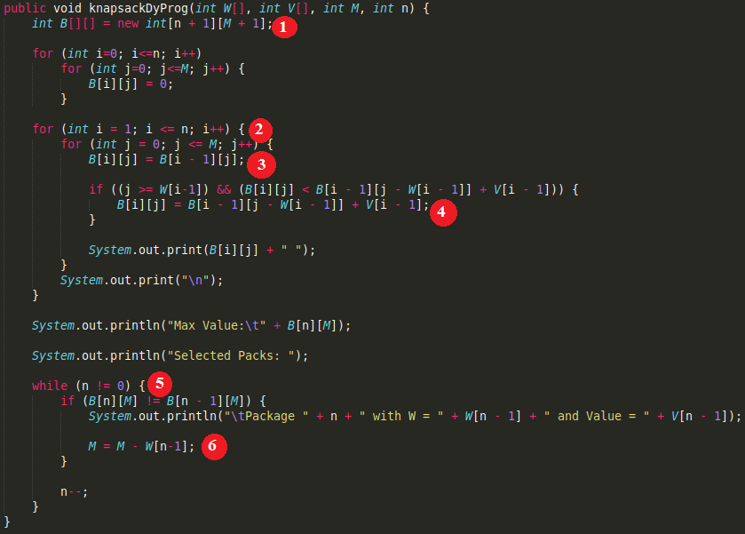
Function knapsackDyProg() in Java

Explanation of the code:

1. Allocate table B[][] and initialize every cell to 0.
2. Fill B[][] bottom-up using the recurrence from the previous section.
3. Start each cell with the “skip package i” value B[i-1][j].
4. If picking package i is feasible and gives a strictly better value, overwrite the cell.
5. Trace the selected items from row n back to row 0.
6. Whenever package n is chosen, decrement the remaining capacity by W[n-1].

Fix note: the original snippet mutated parameter M while still reading B[n][M]. The safer version above uses a separate cursor j for the trace.

The Java driver runs the algorithm on two worked examples:

public void run() {
    // First Example
    // int W[] = new int[]{3, 4, 5, 9, 4};
    // int V[] = new int[]{3, 4, 4, 10, 4};
    // int M = 11;

    // Second Example
    int W[] = new int[]{12, 2, 1, 1, 4};
    int V[] = new int[]{4, 2, 1, 2, 10};
    int M = 15;

    int n = V.length;
    knapsackDyProg(W, V, M, n);
}

Output for the first example:

0 0 0 3 3 3 3 3 3 3 3 3
0 0 0 3 4 4 4 7 7 7 7 7
0 0 0 3 4 4 4 7 7 8 8 8
0 0 0 3 4 4 4 7 7 10 10 10
0 0 0 3 4 4 4 7 8 10 10 11
Max Value:	11
Selected Packs:
	Package 5 with W = 4 and Value = 4
	Package 2 with W = 4 and Value = 4
	Package 1 with W = 3 and Value = 3

Output for the second example:

0 0 0 0 0 0 0 0 0 0 0 0 4 4 4 4
0 0 2 2 2 2 2 2 2 2 2 2 4 4 6 6
0 1 2 3 3 3 3 3 3 3 3 3 4 5 6 7
0 2 3 4 5 5 5 5 5 5 5 5 5 6 7 8
0 2 3 4 10 12 13 14 15 15 15 15 15 15 15 15
Max Value:	15
Selected Packs:
	Package 5 with W = 4 and Value = 10
	Package 4 with W = 1 and Value = 2
	Package 3 with W = 1 and Value = 1
	Package 2 with W = 2 and Value = 2

Time and Space Complexity of 0/1 Knapsack

• Time complexity: O(n · M) — the two nested loops sweep n items across M+1 capacity states.
• Space complexity: O(n · M) for the full table, reducible to O(M) by keeping only the previous row when trace-back is not needed.

The runtime is pseudo-polynomial: polynomial in the value of M but exponential in the bits used to encode M. That is why 0/1 Knapsack remains NP-hard even though Dynamic Programming is efficient in practice.

Applications of the 0/1 Knapsack Problem

• Cargo loading, container packing, and warehouse picking under weight limits.
• Budget allocation across investment projects with fixed cost and expected return.
• Cutting-stock problems in manufacturing that cannot split individual pieces.
• Cryptography schemes such as Merkle-Hellman that build on knapsack hardness.
• Resource-constrained scheduling in cloud computing and CPU task placement.
• Feature selection in machine learning under a fixed feature budget.

FAQs