
Travelling Salesman Problem: Python, C++ Algorithm
 Editorial Team
⚡ Smart Summary
Travelling Salesman Problem is a classic NP-hard optimization task that asks for the shortest tour that visits every city exactly once and returns to the origin, using distance data supplied through a graph.
What is the Travelling Salesman Problem (TSP)?
The Travelling Salesman Problem (TSP) is a classic combinatorial optimization problem in theoretical computer science. Given a graph of cities, TSP asks for the shortest path that visits every node exactly once and returns to the origin city.
The problem statement provides a list of cities along with the distances between each pair of cities.
Objective: Start at the origin city, visit every other city exactly once, and return to the starting city. The target is to find the shortest possible round-trip route.
Example of TSP
Consider the graph below where 1, 2, 3, and 4 represent the cities, and the weight on every edge represents the distance between those cities.
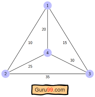
The goal is to find the shortest possible tour that starts from the origin city, visits every other city exactly once, and returns to the origin city.
For the graph above, the optimal route is 1-2-4-3-1. The shortest tour cost is 10 + 25 + 30 + 15 = 80.
Different Solutions to Travelling Salesman Problem

The Travelling Salesman Problem is classified as NP-hard because no known polynomial-time algorithm solves it exactly. The complexity grows exponentially with the number of cities.
There are multiple ways to attack TSP. The most common approaches are:
Brute Force Approach: The naive method calculates every possible tour and compares them. The number of tours in a graph with n cities is n!, which makes brute force computationally very expensive for anything beyond about ten cities.
Branch and Bound Method: The problem is broken into sub-problems, and the solutions of those sub-problems combine into an optimal solution. Effective pruning discards partial tours that cannot beat the current best cost.
This tutorial demonstrates the dynamic programming approach, which is the memoized version of branch and bound and matches the Bellman-Held-Karp algorithm.
Dynamic Programming: This is an exact method that seeks the optimal solution by reusing overlapping subproblem results. It is slower than the near-optimal greedy methods, but it always returns a globally optimal tour.
The computational complexity of this approach is O(N² × 2^N), which we discuss later in the article.
Nearest Neighbour Method: A heuristic greedy approach that always jumps to the nearest unvisited city. It is much cheaper than dynamic programming but does not guarantee an optimal tour, so it is used for near-optimal solutions when speed matters more than exact minima.
Algorithm for Traveling Salesman Problem
We use the dynamic programming approach to solve TSP. Before starting the algorithm, let us settle a few terminologies:
- A graph
G = (V, E)is a set of vertices and edges. Vis the set of vertices.Eis the set of edges.- Vertices are connected through edges.
Dist(i, j)denotes the non-negative distance between vertices i and j.
Assume S is a subset of cities drawn from {1, 2, 3, …, n} where i and j are two cities in that subset. Then cost(i, S, j) is the length of the shortest path that starts at i, visits every city in S exactly once, and ends at j.
For example, cost(1, {2, 3, 4}, 1) denotes the shortest path where:
- Starting city is 1
- Cities 2, 3, and 4 are visited only once
- The ending point is 1
The dynamic programming recurrence is:
- Set
cost(i, {}, i) = 0, which means we start and end at i with zero cost. - When
|S| > 1, definecost(i, S, 1) = ∞fori ≠ 1, because the true tour cost is unknown yet. - Starting at city 1, choose the next city so that
cost(i, S, j) = min [ cost(i, S − {i}, j) + dist(i, j) ]fori ∈ Sandi ≠ j.
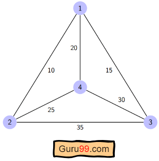
For the graph above, the adjacency matrix is the following:
| dist(i, j) | 1 | 2 | 3 | 4 |
|---|---|---|---|---|
| 1 | 0 | 10 | 15 | 20 |
| 2 | 10 | 0 | 35 | 25 |
| 3 | 15 | 35 | 0 | 30 |
| 4 | 20 | 25 | 30 | 0 |
Here is how the algorithm proceeds:
Step 1) The journey starts at city 1, visits every other city once, and returns to city 1.
Step 2) S is a subset of cities. For every |S| > 1, initialise cost(i, S, 1) = ∞. Here cost(i, S, j) denotes a tour that starts at i, visits the cities in S once, and reaches j. We start from infinity because the distance is unknown at this point. So the values are:
cost(2, {3, 4}, 1) = ∞ means we start at city 2, go through cities 3 and 4, and reach 1, with unknown cost. Similarly:
cost(3, {2, 4}, 1) = ∞
cost(4, {2, 3}, 1) = ∞
Step 3) For every subset of S, compute:
cost(i, S, j) = min [ cost(i, S − {i}, j) + dist(i, j) ], where j ∈ S and i ≠ j.
That is the minimum cost tour that starts at i, visits the subset of cities once, and returns to j. Because the tour starts at city 1, the optimal cost is cost(1, {other cities}, 1).
Working the Recurrence Step by Step
Now S = {1, 2, 3, 4}. There are four elements, so the number of subsets is 2^4 = 16. Those subsets are:
1) |S| = 0: {Φ}
2) |S| = 1: {{1}, {2}, {3}, {4}}
3) |S| = 2: {{1, 2}, {1, 3}, {1, 4}, {2, 3}, {2, 4}, {3, 4}}
4) |S| = 3: {{1, 2, 3}, {1, 2, 4}, {2, 3, 4}, {1, 3, 4}}
5) |S| = 4: {{1, 2, 3, 4}}
Because the tour starts at city 1, we can discard every subset that contains city 1 while computing intermediate costs.
The algorithm calculation unfolds as follows:
1) |S| = Φ:
- cost(2, Φ, 1) = dist(2, 1) = 10
- cost(3, Φ, 1) = dist(3, 1) = 15
- cost(4, Φ, 1) = dist(4, 1) = 20
2) |S| = 1:
- cost(2, {3}, 1) = dist(2, 3) + cost(3, Φ, 1) = 35 + 15 = 50
- cost(2, {4}, 1) = dist(2, 4) + cost(4, Φ, 1) = 25 + 20 = 45
- cost(3, {2}, 1) = dist(3, 2) + cost(2, Φ, 1) = 35 + 10 = 45
- cost(3, {4}, 1) = dist(3, 4) + cost(4, Φ, 1) = 30 + 20 = 50
- cost(4, {2}, 1) = dist(4, 2) + cost(2, Φ, 1) = 25 + 10 = 35
- cost(4, {3}, 1) = dist(4, 3) + cost(3, Φ, 1) = 30 + 15 = 45
3) |S| = 2:
- cost(2, {3, 4}, 1) = min [ dist(2, 3) + cost(3, {4}, 1) = 35 + 50 = 85, dist(2, 4) + cost(4, {3}, 1) = 25 + 45 = 70 ] = 70
- cost(3, {2, 4}, 1) = min [ dist(3, 2) + cost(2, {4}, 1) = 35 + 45 = 80, dist(3, 4) + cost(4, {2}, 1) = 30 + 35 = 65 ] = 65
- cost(4, {2, 3}, 1) = min [ dist(4, 2) + cost(2, {3}, 1) = 25 + 50 = 75, dist(4, 3) + cost(3, {2}, 1) = 30 + 45 = 75 ] = 75
4) |S| = 3:
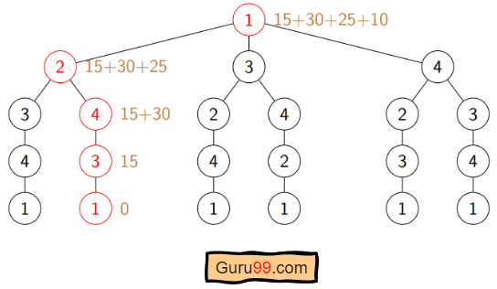
- cost(1, {2, 3, 4}, 1) = min [ dist(1, 2) + cost(2, {3, 4}, 1) = 10 + 70 = 80, dist(1, 3) + cost(3, {2, 4}, 1) = 15 + 65 = 80, dist(1, 4) + cost(4, {2, 3}, 1) = 20 + 75 = 95 ] = 80
So the optimal solution is 1-2-4-3-1.
Pseudo-code
Algorithm: Traveling-Salesman-Problem
Cost (1, {}, 1) = 0
for s = 2 to n do
    for all subsets S belongs to {1, 2, 3, ..., n} of size s
        Cost (s, S, 1) = Infinity
    for all i in S and i != 1
        Cost (i, S, j) = min {Cost (i, S - {i}, j) + dist(i, j) for j in S and i != j}
Return min(i) Cost (i, {1, 2, 3, ..., n}, j) + d(j, i)
Implementation in C/C++
Here is the implementation in C++. The version below fixes the source’s early return bug, which returned after the very first permutation instead of enumerating all tours.
#include <bits/stdc++.h>
using namespace std;
#define V 4
#define MAX 1000000

int tsp(int graph[][V], int s) {
    vector<int> vertex;
    for (int i = 0; i < V; i++)
        if (i != s)
            vertex.push_back(i);

    int min_cost = MAX;
    do {
        int current_cost = 0;
        int j = s;
        for (int i = 0; i < vertex.size(); i++) {
            current_cost += graph[j][vertex[i]];
            j = vertex[i];
        }
        current_cost += graph[j][s];
        min_cost = min(min_cost, current_cost);
    } while (next_permutation(vertex.begin(), vertex.end()));

    return min_cost;
}

int main() {
    int graph[][V] = {
        { 0, 10, 15, 20 },
        { 10, 0, 35, 25 },
        { 15, 35, 0, 30 },
        { 20, 25, 30, 0 }
    };
    int s = 0;
    cout << tsp(graph, s) << endl;
    return 0;
}
Output:
80
Implementation in Python
The Python implementation mirrors the C++ version. It corrects the source’s from itertools, import comma typo, the misplaced return inside the inner loop, and the stray indent on s = 0.
from sys import maxsize
from itertools import permutations

V = 4

def tsp(graph, s):
    vertex = []
    for i in range(V):
        if i != s:
            vertex.append(i)

    min_cost = maxsize
    for perm in permutations(vertex):
        current_cost = 0
        k = s
        for j in perm:
            current_cost += graph[k][j]
            k = j
        current_cost += graph[k][s]
        min_cost = min(min_cost, current_cost)
    return min_cost

graph = [[0, 10, 15, 20],
         [10, 0, 35, 25],
         [15, 35, 0, 30],
         [20, 25, 30, 0]]
s = 0
print(tsp(graph, s))
Output:
80
Academic Solutions to TSP
Computer scientists have spent decades searching for improved polynomial-time algorithms for the Travelling Salesman Problem. So far, TSP remains NP-hard.
Several published techniques reduce the practical complexity for specific families of TSP instances:
- The classical symmetric TSP is solved by the Zero Suffix Method.
- The Biogeography-based Optimization Algorithm uses migration strategies to solve optimization problems that map to TSP.
- The Multi-Objective Evolutionary Algorithm is designed for multi-objective TSP and builds on NSGA-II.
- The Multi-Agent System approach solves TSP for N cities with fixed computational resources.
- The Lin-Kernighan heuristic and its successor LKH deliver tours within 2-3% of the optimum for instances with millions of cities.
- Concorde uses cutting planes and branch-and-cut to compute exact optima for benchmark instances with tens of thousands of cities.
Application of Traveling Salesman Problem
The Travelling Salesman Problem shows up in the real world in both pure and modified forms. Some of the main applications are:
- Planning, logistics, and microchip manufacturing: Chip insertion problems in the microchip industry are modelled as TSP variants to minimise robot arm travel time.
- DNA sequencing: A modified TSP is used in DNA sequencing where cities represent DNA fragments and distances represent similarity between fragments.
- Astronomy: Astronomers use TSP to minimise the time spent slewing telescopes between observation targets.
- Optimal control: TSP formulations model optimal-control problems where multiple constraints must be honoured while minimising traversal cost.
- Last-mile delivery: Amazon, UPS, and food delivery apps solve dynamic TSP variants to sequence stops for drivers.
- Warehouse picking: Robotic and human pickers follow TSP-optimised routes that shorten travel time inside distribution centres.
Complexity Analysis of TSP
- Time Complexity: The Held-Karp dynamic programming approach solves 2N subsets for each starting node, giving
N × 2^Nsubproblems. Each subproblem takes linear time to combine. If the origin node is unspecified, an outer loop over N nodes is required. The total time complexity isO(N² × 2^N). - Space Complexity: The DP table stores
C(S, i)for each subset S of the vertex set. There are 2N subsets per node, so the space complexity isO(N × 2^N), which is often written asO(2^N)when N is treated as fixed.
Next, learn about the Sieve of Eratosthenes Algorithm.
