
Data Validation in Excel: Filters, Grouping, Sorting Examples
 Charlotte Miller
⚡ Smart Summary
Data Validation in Excel restricts what a cell accepts, while filters, sorting, and grouping organise the records around it. This page explains validation rules with error alerts, text and number filters, sorting, grouping with subtotals, and inserting images into a worksheet.

Data validation
Data validation is very important in the sense that it helps us avoid mistakes that can be avoided. Let’s assume you are recording student exam marks and you know the minimum is 0 and the maximum is 100. You can take advantage of validation features to ensure that only values between 0 and 100 are entered.
Add a new sheet in your workbook by clicking on the plus button at the bottom of the worksheet.
Add a column for S/N, Name and Score. Your sheet should look as follows
| S/N | Name | Score |
|---|---|---|
| 1 | Jane | |
| 2 | James | |
| 3 | Jones | |
| 4 | Jonathan | |
| 5 | John |
- Click on the DATA tab
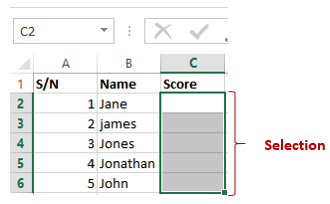
- Select the cells C2 to C6 (The cells that will be used to record the scores)
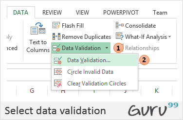
- Click on Data validation drop down list.
- Click on Data validation.
- You will get the following dialogue window

- Click on Error Alert tab
- Enter the alert title and message as shown in the diagram below.

- Click on OK button
- Try to enter a score greater than 200. You will get the following error message

Data Validation Criteria Types
The Allow drop down of the Data Validation window offers several criteria, not only whole numbers. Choosing the right one keeps the entries clean at the point of typing. The table below lists the common criteria with a practical example.
| Criterion | What it allows | Example |
|---|---|---|
| Whole number | Integers within a range | Between 0 and 100 for an exam score |
| Decimal | Numbers with decimals within a range | Between 0 and 1 for a discount rate |
| List | Only values from a defined list, shown as a drop down | Male, Female |
| Date | Dates within a range | On or after today |
| Text length | A limited number of characters | Exactly 10 for a phone number |
| Custom | Any formula that returns TRUE or FALSE | =ISNUMBER(C2) to force a number |
💡 Tip: Use the Input Message tab to show a hint when the cell is selected, and the Error Alert tab to decide whether a wrong entry is a hard Stop, a Warning that can be overridden, or an Information note.
Data filters
Data filters allow us to get data that matches our desired criteria. Let’s say we want to show the results of all the students whose names start with “ja” or get scores that are less than, greater than or equal to a certain value, we can use filters to get such data.
Select the name and scores columns as shown below

- Click on DATA tab on the ribbon
- Click on Sort & Filter drop down list as shown in the image below

- Click on the Name Filter
- Select text filters
- Select begins with
- You will get the following window.

- Enter “ja” and click on “OK” button
- You should be able to see only the results for Jane and James.

Sorting Data in Excel
Filtering hides the rows that do not match, while sorting keeps every row but changes their order. Sorting the student scores from the highest to the lowest makes the ranking obvious at a glance, and it is another command on the DATA tab.
- Select a cell in the column: Click any cell in the Score column. There is no need to highlight the whole column, because Excel detects the surrounding table.
- Open Sort & Filter: On the DATA tab, choose Sort Largest to Smallest for numbers, or Sort A to Z for text.
- Sort by several columns: For a multi level sort, click the Sort button, add a level, and sort first by Gender and then by Score. Excel applies the levels from top to bottom.
- Keep the header: Make sure “My data has headers” is ticked, so the column names stay in place and are not sorted with the data.
⚠️ Warning: Select only one cell, never a single column, before sorting. If just one column is highlighted and sorted, the names and scores are separated and the record is corrupted. Excel warns with an “Expand the selection” prompt, which should always be accepted.
Group and Ungroup
Groups allow us to view easily and hide unnecessary details from either columns or rows. In addition to that, we can also use groups to analyse data that belongs to a common category. Let’s illustrate this with an example. We will use the student scores example above.

- Right click on the score and select insert column. Name the name column gender.
- Change James to Juanita. Put female for Janet and Juanita. Put male for the rest of the students. Your sheet should look as follows.

We will now group the females together and display their average score and do the same for the males.
- Click on DATA tab on the ribbon
- Select all the columns and rows with data
- Click on Group drop down button as shown in the image below

You will get the following window

- Make sure Rows options is selected
- Click on OK button
- You will get the following preview

- We will now calculate the average scores for females and males
- Select the whole data as shown below

Click on Subtotal drop down button under DATA tab

You will get the following window

- Set “At each change” into gender
- Set “Use function” to average
- Select “Add subtotal” to Score
- Click on “OK” button

Adding images to spreadsheets
At times, you would like to brand the documents printed in excel with letterhead information and print with the company logo, etc. Excel has features that allow you to import images into Excel. The command for adding images is found under the INSERT tab on the ribbon.

You will get the following dialogue window

- You can browse to any folder on your computer that has pictures, and you can select any picture of your choice.
- You will get results similar to the ones shown below

Tutorial exercise 4
Use the INSERT tab pictures command to add a picture of your choice to the worksheet.
