
How to Do Addition, Subtraction, Multiplication & Division in Excel
 Charlotte Miller
⚡ Smart Summary
Addition, subtraction, multiplication, and division in Excel start with the equal sign and cell references such as =C2+D2. This page explains the four arithmetic operators, the order of operations, equivalent functions, formatting, print setup, and common formula errors.

How To Perform Arithmetic Operations in Excel
In this tutorial, we are going to perform basic arithmetic operations i.e. addition, subtraction, division and multiplication. The following table shows the data that we will work with and the results that we should expect.
| S/N | ARITHMETIC OPERATOR | FIRST NUMBER | SECOND NUMBER | RESULT |
|---|---|---|---|---|
| 1 | Addition (+) | 13 | 3 | 16 |
| 2 | Subtraction (-) | 21 | 9 | 12 |
| 3 | Division (/) | 33 | 12 | 2.75 |
| 4 | Multiplication (*) | 7 | 3 | 21 |
Let’s now use Microsoft excel to achieve the above results
Step 1) Create an Excel Sheet and Enter the Data
Create a folder on your computer in my documents folder and name it Guru99 Excel Tutorials
For this tutorial, we will be using Microsoft Excel 2013. The good news is even if you have Microsoft Excel 2007 or 2010, you will still be able to follow the tutorial and get the same result.
Open Excel. You will get a window similar to the one shown below. The outlook of Excel will depend on your version.

- Enter the data in your worksheet as shown in the image above.
- We will now perform the calculations using the respective arithmetic operators. When performing calculations in Excel, you should always start with the equal (=) sign.
- Let’s start with the one for addition. Write the following formula in E2 Excel (Result column)
- =C2+D2
HERE,
- “=” tells Excel to evaluate whatever follows after the equal sign
- “C2” is the cell address of the first number given by C representing the column letter and 2 representing the row number
- “D2” is the cell address of the second number given by D representing the column letter and 2 representing the row number
Press enter key on the keyboard when done. You should get 16 as the result.
Using the knowledge gained in the above example, try to write the formulas for subtraction, division, and multiplication.
Step 2) Format Data in Microsoft Excel
We all love beautiful things don’t we? Formatting in Excel helps us achieve exactly that. We can make our spreadsheets more presentable. We will use the data in the arithmetic operations table. We will make the column names;
- Bold
- Align serial numbers to the left
- Enclose the data in boxes.
Step 3) Make Column Names Bold
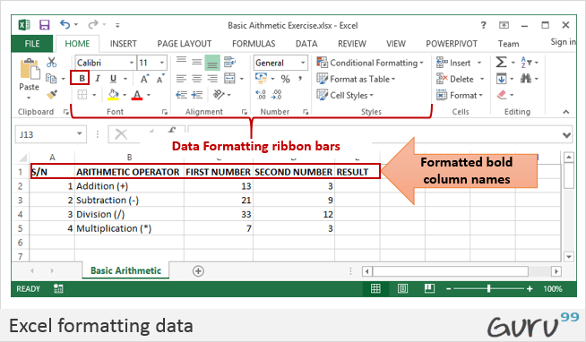
- Highlight the cells that have the column names by dragging them.
- Click on the bold button represented by B command.
- Your workbook should now appear as follows
Step 4) Align Data to the Left
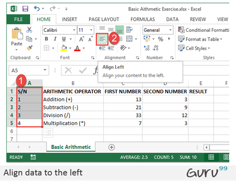
- We will align the serial numbers to the left
- Highlight all the data in the S/N column
- Click on align left as shown below
Step 5) Enclose Data in Boxes
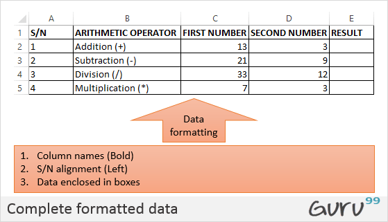
Highlight all the columns and rows with data
On the font ribbon bar, click on borders command as shown below.

You will get the following drop down menu

Select the option “All Borders”.
Your data should now look as follows
Using the knowledge gained above, try to change the font color and try out other options available on the Home tab.
Step 6) Set the Print Area, Print Preview & Page Layout
The print area is the part of the worksheet that you would like to print out on paper. The quick and easy way of doing it is by using the following shortcut commands
Ctrl + P
You will get the following print preview.

Press Esc button to exit print preview mode
The page setup ribbon bar has a number of options i.e. orientation, size, etc. Try to apply the different settings and use Ctrl + P shortcut to preview the effects on the worksheet.
Excel Arithmetic Operators and Order of Operations
Every calculation above uses one of the four arithmetic operators. Knowing the exact symbol and, just as important, the order in which Excel applies them, prevents the most common mistakes. The table below lists the operators with an example based on the data used earlier.
| Operation | Operator | Example formula | Result |
|---|---|---|---|
| Addition | + | =C2+D2 | 16 |
| Subtraction | – | =C3-D3 | 12 |
| Division | / | =C4/D4 | 2.75 |
| Multiplication | * | =C5*D5 | 21 |
When a formula mixes several operators, Excel does not read it from left to right. It follows the BODMAS rule, which means Brackets first, then Orders (powers), then Division and Multiplication, and finally Addition and Subtraction. For example, =2+3*4 returns 14, because the multiplication runs before the addition. To force the addition first, add brackets: =(2+3)*4 returns 20. Whenever the result looks wrong, adding brackets is the quickest fix.
Using Functions Instead of Operators
Operators are ideal for two or three numbers, but a function is faster and cleaner when many cells are involved. Excel offers a built in function for each of the four operations, and they accept a range of cells.
- SUM adds a range. Instead of =C2+C3+C4+C5, write =SUM(C2:C5).
- PRODUCT multiplies a range. =PRODUCT(C5,D5) returns the same 21 as =C5*D5.
- Subtraction has no dedicated function, so it is expressed as an addition of a negative value, for example =SUM(C3,-D3).
- QUOTIENT returns only the whole part of a division, so =QUOTIENT(33,12) returns 2, while =33/12 returns 2.75.
A short worked example ties them together. Suppose the numbers 13, 21, 33, and 7 sit in cells C2 to C5. The formula =SUM(C2:C5) returns 74, and =PRODUCT(C2:C5) returns 63063. The main advantage is that a function keeps working when rows are inserted into the range, whereas a long chain of plus signs has to be edited by hand.
💡 Tip: Select a range of numbers and read the total, average, and count on the status bar at the bottom right of the Excel window. It is the fastest way to check a result without writing any formula.
Common Excel Formula Errors
When a formula cannot be calculated, Excel shows an error code in the cell instead of a value. Recognising the four most common codes makes them quick to fix.
| Error | Meaning | Typical fix |
|---|---|---|
| #DIV/0! | A number is divided by zero or by an empty cell | Check the divisor, or wrap the formula in IFERROR |
| #VALUE! | A formula refers to text where a number is expected | Make sure every referenced cell holds a number |
| #NAME? | A function name or a range name is spelled wrong | Correct the spelling, for example SUM not SUmM |
| #REF! | A referenced cell was deleted | Undo the deletion or point the formula at a valid cell |
⚠️ Warning: A very long number may show as ##### in a cell. This is not an error, it only means the column is too narrow. Widen the column, and the value appears in full.
