Excel Formulas & Functions with Basic Examples
⚡ Smart Summary
Formulas and Functions in Excel are the building blocks for working with numeric data. This page explains how a formula operates on cell references and operators, how a built in function shortens the work, and it covers statistical, numeric, string, date, and VLOOKUP functions.
Formulas and functions are the building blocks of working with numeric data in Excel. This article introduces you to formulas and functions.
Tutorials Data
For this tutorial, we will work with the following datasets.
Home supplies budget
| S/N | ITEM | QTY | PRICE | SUBTOTAL | Is it Affordable? |
|---|---|---|---|---|---|
| 1 | Mangoes | 9 | 600 | ||
| 2 | Oranges | 3 | 1200 | ||
| 3 | Tomatoes | 1 | 2500 | ||
| 4 | Cooking Oil | 5 | 6500 | ||
| 5 | Tonic Water | 13 | 3900 |
House Building Project Schedule
| S/N | ITEM | START DATE | END DATE | DURATION (DAYS) |
|---|---|---|---|---|
| 1 | Survey land | 04/02/2015 | 07/02/2015 | |
| 2 | Lay Foundation | 10/02/2015 | 15/02/2015 | |
| 3 | Roofing | 27/02/2015 | 03/03/2015 | |
| 4 | Painting | 09/03/2015 | 21/03/2015 |
What is Formulas in Excel?
FORMULAS IN EXCEL is an expression that operates on values in a range of cell addresses and operators. For example, =A1+A2+A3, which finds the sum of the range of values from cell A1 to cell A3. An example of a formula made up of discrete values like =6*3.
=A2 * D2 / 2
HERE,
"="tells Excel that this is a formula, and it should evaluate it."A2" * D2"makes reference to cell addresses A2 and D2 then multiplies the values found in these cell addresses."/"is the division arithmetic operator"2"is a discrete value
Formulas practical exercise
We will work with the sample data for the home budget to calculate the subtotal.
- Create a new workbook in Excel
- Enter the data shown in the home supplies budget above.
- Your worksheet should look as follows.
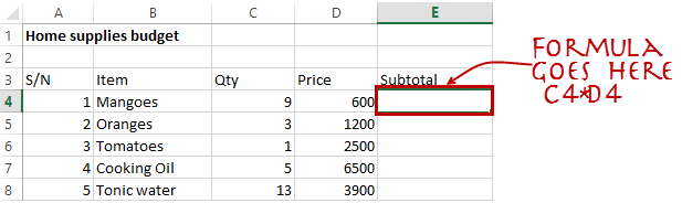
We will now write the formula that calculates the subtotal
Set the focus to cell E4
Enter the following formula.
=C4*D4
HERE,
"C4*D4"uses the arithmetic operator multiplication (*) to multiply the value of the cell address C4 and D4.
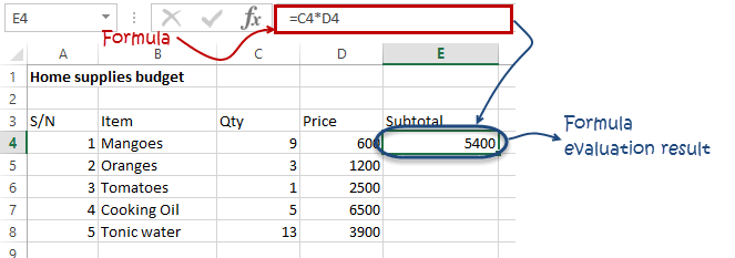
Press enter key
You will get the following result
The following animated image shows you how to auto select cell address and apply the same formula to other rows.
Mistakes to avoid when working with formulas in Excel
- Remember the rules of Brackets of Division, Multiplication, Addition, & Subtraction (BODMAS). This means expressions are brackets are evaluated first. For arithmetic operators, the division is evaluated first followed by multiplication then addition and subtraction is the last one to be evaluated. Using this rule, we can rewrite the above formula as =(A2 * D2) / 2. This will ensure that A2 and D2 are first evaluated then divided by two.
- Excel spreadsheet formulas usually work with numeric data; you can take advantage of data validation to specify the type of data that should be accepted by a cell i.e. numbers only.
- To ensure that you are working with the correct cell addresses referenced in the formulas, you can press F2 on the keyboard. This will highlight the cell addresses used in the formula, and you can cross check to ensure they are the desired cell addresses.
- When you are working with many rows, you can use serial numbers for all the rows and have a record count at the bottom of the sheet. You should compare the serial number count with the record total to ensure that your formulas included all the rows.
Check Out
Top 10 Excel Spreadsheet Formulas
What is Function in Excel?
FUNCTION IN EXCEL is a predefined formula that is used for specific values in a particular order. Function is used for quick tasks like finding the sum, count, average, maximum value, and minimum values for a range of cells. For example, cell A3 below contains the SUM function which calculates the sum of the range A1:A2.
- SUM for summation of a range of numbers
- AVERAGE for calculating the average of a given range of numbers
- COUNT for counting the number of items in a given range
The importance of functions
Functions increase user productivity when working with excel. Let’s say you would like to get the grand total for the above home supplies budget. To make it simpler, you can use a formula to get the grand total. Using a formula, you would have to reference the cells E4 through to E8 one by one. You would have to use the following formula.
= E4 + E5 + E6 + E7 + E8
With a function, you would write the above formula as
=SUM (E4:E8)
As you can see from the above function used to get the sum of a range of cells, it is much more efficient to use a function to get the sum than using the formula which will have to reference a lot of cells.
Common functions
Let’s look at some of the most commonly used functions in ms excel formulas. We will start with statistical functions.
| S/N | FUNCTION | CATEGORY | DESCRIPTION | USAGE |
|---|---|---|---|---|
| 01 | SUM | Math & Trig | Adds all the values in a range of cells | =SUM(E4:E8) |
| 02 | MIN | Statistical | Finds the minimum value in a range of cells | =MIN(E4:E8) |
| 03 | MAX | Statistical | Finds the maximum value in a range of cells | =MAX(E4:E8) |
| 04 | AVERAGE | Statistical | Calculates the average value in a range of cells | =AVERAGE(E4:E8) |
| 05 | COUNT | Statistical | Counts the number of cells in a range of cells | =COUNT(E4:E8) |
| 06 | LEN | Text | Returns the number of characters in a string text | =LEN(B7) |
| 07 | SUMIF | Math & Trig | Adds all the values in a range of cells that meet a specified criteria. =SUMIF(range,criteria,[sum_range]) |
=SUMIF(D4:D8,”>=1000″,C4:C8) |
| 08 | AVERAGEIF | Statistical | Calculates the average value in a range of cells that meet the specified criteria. =AVERAGEIF(range,criteria,[average_range]) |
=AVERAGEIF(F4:F8,”Yes”,E4:E8) |
| 09 | DAYS | Date & Time | Returns the number of days between two dates | =DAYS(D4,C4) |
| 10 | NOW | Date & Time | Returns the current system date and time | =NOW() |
Numeric Functions
As the name suggests, these functions operate on numeric data. The following table shows some of the common numeric functions.
| S/N | FUNCTION | CATEGORY | DESCRIPTION | USAGE |
|---|---|---|---|---|
| 1 | ISNUMBER | Information | Returns True if the supplied value is numeric and False if it is not numeric | =ISNUMBER(A3) |
| 2 | RAND | Math & Trig | Generates a random number between 0 and 1 | =RAND() |
| 3 | ROUND | Math & Trig | Rounds off a decimal value to the specified number of decimal points | =ROUND(3.14455,2) |
| 4 | MEDIAN | Statistical | Returns the number in the middle of the set of given numbers | =MEDIAN(3,4,5,2,5) |
| 5 | PI | Math & Trig | Returns the value of Math Function PI(π) | =PI() |
| 6 | POWER | Math & Trig | Returns the result of a number raised to a power. POWER( number, power ) |
=POWER(2,4) |
| 7 | MOD | Math & Trig | Returns the Remainder when you divide two numbers | =MOD(10,3) |
| 8 | ROMAN | Math & Trig | Converts a number to roman numerals | =ROMAN(1984) |
String functions
These basic excel functions are used to manipulate text data. The following table shows some of the common string functions.
| S/N | FUNCTION | CATEGORY | DESCRIPTION | USAGE | COMMENT |
|---|---|---|---|---|---|
| 1 | LEFT | Text | Returns a number of specified characters from the start (left-hand side) of a string | =LEFT(“GURU99”,4) | Left 4 Characters of “GURU99” |
| 2 | RIGHT | Text | Returns a number of specified characters from the end (right-hand side) of a string | =RIGHT(“GURU99”,2) | Right 2 Characters of “GURU99” |
| 3 | MID | Text | Retrieves a number of characters from the middle of a string from a specified start position and length. =MID (text, start_num, num_chars) |
=MID(“GURU99”,2,3) | Retrieving Characters 2 to 5 |
| 4 | ISTEXT | Information | Returns True if the supplied parameter is Text | =ISTEXT(value) | value – The value to check. |
| 5 | FIND | Text | Returns the starting position of a text string within another text string. This function is case-sensitive. =FIND(find_text, within_text, [start_num]) |
=FIND(“oo”,”Roofing”,1) | Find oo in “Roofing”, Result is 2 |
| 6 | REPLACE | Text | Replaces part of a string with another specified string. =REPLACE (old_text, start_num, num_chars, new_text) |
=REPLACE(“Roofing”,2,2,”xx”) | Replace “oo” with “xx” |
Date Time Functions
These functions are used to manipulate date values. The following table shows some of the common date functions
| S/N | FUNCTION | CATEGORY | DESCRIPTION | USAGE |
|---|---|---|---|---|
| 1 | DATE | Date & Time | Returns the number that represents the date in excel code | =DATE(2015,2,4) |
| 2 | DAYS | Date & Time | Find the number of days between two dates | =DAYS(D6,C6) |
| 3 | MONTH | Date & Time | Returns the month from a date value | =MONTH(“4/2/2015”) |
| 4 | MINUTE | Date & Time | Returns the minutes from a time value | =MINUTE(“12:31”) |
| 5 | YEAR | Date & Time | Returns the year from a date value | =YEAR(“04/02/2015”) |
VLOOKUP function
The VLOOKUP function is used to perform a vertical look up in the left most column and return a value in the same row from a column that you specify. Let’s explain this in a layman’s language. The home supplies budget has a serial number column that uniquely identifies each item in the budget. Suppose you have the item serial number, and you would like to know the item description, you can use the VLOOKUP function. Here is how the VLOOKUP function would work.
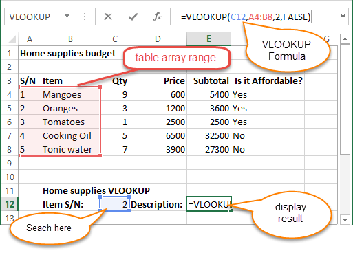
=VLOOKUP (C12, A4:B8, 2, FALSE)
HERE,
"=VLOOKUP"calls the vertical lookup function"C12"specifies the value to be looked up in the left most column"A4:B8"specifies the table array with the data"2"specifies the column number with the row value to be returned by the VLOOKUP function"FALSE,"tells the VLOOKUP function that we are looking for an exact match of the supplied look up value
The animated image below shows this in action
Here is a list of important Excel Formula and Function
- SUM function =
=SUM(E4:E8) - MIN function =
=MIN(E4:E8) - MAX function =
=MAX(E4:E8) - AVERAGE function =
=AVERAGE(E4:E8) - COUNT function =
=COUNT(E4:E8) - DAYS function =
=DAYS(D4,C4) - VLOOKUP function =
=VLOOKUP (C12, A4:B8, 2, FALSE) - DATE function =
=DATE(2020,2,4)