Excel VLOOKUP Tutorial for Beginners
⚡ Smart Summary
Excel VLOOKUP Tutorial explains how the vertical lookup function searches the first column of a table and returns a matching value from another column. This guide covers syntax, exact and approximate matches, cross-sheet lookups, common errors, and the modern XLOOKUP alternative.

What is VLOOKUP?
VLOOKUP (the V stands for Vertical) is a built-in Excel function that establishes a relationship between columns in a spreadsheet. It allows you to look up a value in one column and return the corresponding value from another column in the same row.
VLOOKUP Syntax and Arguments
Before applying VLOOKUP, it helps to understand the formula structure. The function takes four arguments and follows a consistent pattern across every Excel version.
- lookup_value — the value you want to find (a cell reference or literal).
- table_array — the range of cells containing the lookup column and return column.
- col_index_num — the column number in table_array from which to return the value (1 is the leftmost).
- range_lookup — FALSE for an exact match, TRUE (or omitted) for an approximate match on sorted data.
Important: The lookup value must sit in the leftmost column of table_array, and VLOOKUP only searches left to right.
Usage of VLOOKUP
When you need to find specific information in a large spreadsheet, or to retrieve the same kind of value repeatedly, VLOOKUP saves significant time compared to manual filtering.
Consider a Company Salary Table maintained by the finance team. You start with a known piece of information — an index — and use VLOOKUP to fetch the unknown value.
For example, you already know the Employee Name:

And you want to look up the Employee Salary:

Excel spreadsheet for the above instance:
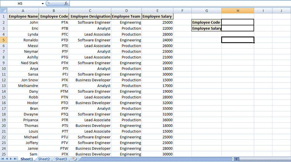
To find the unknown Employee Salary, we enter the Employee Code that is already available.

By applying VLOOKUP, the salary value corresponding to that Employee Code appears automatically.
How to use VLOOKUP function in Excel
Follow this step-by-step guide to apply the VLOOKUP function in Excel:
Step 1) Navigate to the target cell
Click the cell where you want the salary of the selected employee to appear — in this example, cell H3.

Step 2) Enter the VLOOKUP function =VLOOKUP()
Type the function in the cell. Begin with an equal sign (which tells Excel a formula follows) and then the VLOOKUP keyword: =VLOOKUP().

The parentheses contain the set of arguments (the pieces of data the function needs).
VLOOKUP requires four arguments:
Step 3) First Argument — the lookup value
The first argument is the cell reference for the value you want to search for. In this case, the Employee Code is the lookup value, so the first argument is H2 — the cell whose contents Excel should match.

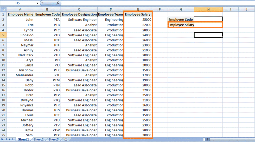
Step 4) Second Argument — the table array
This refers to the block of values to be searched, known in Excel as the table array or lookup table. In our example, the lookup table runs from B2 to E25.
NOTE: The lookup column must be the leftmost column of your table array.

Step 5) Third Argument — col_index_num
This tells VLOOKUP which column inside the table array holds the return value. The Employee Salary sits in the fourth column, so the column index is 4.

Step 6) Fourth Argument — exact or approximate match
The last argument is the range lookup flag. It controls whether VLOOKUP returns an exact or an approximate match. Here we want an exact match (FALSE).
- FALSE — exact match.
- TRUE — approximate match.

Step 7) Press Enter
Press Enter to complete the formula. You will see an error initially because no Employee Code has been entered in H2 yet.

Once you enter a valid Employee Code in H2, the cell returns the corresponding Employee Salary.

In short, the formula tells Excel that the known values sit in the leftmost column of the data (Employee Code). VLOOKUP then scans the table and returns the fourth-column value on the matching row — the Employee Salary.
This example covered exact matches (the FALSE keyword). The next section explains approximate matches.
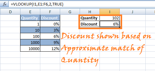
VLOOKUP for Approximate Matches (TRUE Keyword as the last parameter)
Consider a scenario in which a table calculates discounts for customers who do not purchase exactly tens or hundreds of items.
As shown below, a company applies discounts to quantities ranging from 1 to 10,000:
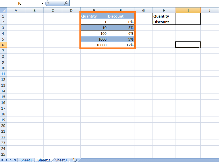
A customer rarely buys exactly 100 or 1,000 units. The approximate-match mode lets VLOOKUP find the closest lower value rather than insisting on an exact figure. Steps:
Step 1) Click the cell where the VLOOKUP function will go — cell reference I2.

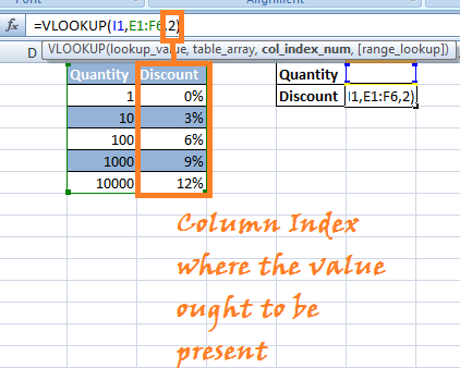
Step 2) Enter =VLOOKUP() in the cell and add the arguments inside the parentheses.

Step 3) Argument 1: Enter the cell reference whose value should be matched against the lookup table.

Step 4) Argument 2: Select the lookup table — here, the Quantity and Discount columns.

Step 5) Argument 3: Enter the column index in the lookup table from which to return the matching value.
Step 6) Argument 4: Set the last argument to TRUE for approximate matches.

Step 7) Press Enter. The formula now applies to the cell. When you type any quantity, Excel returns the discount band based on the approximate match.
NOTE: If you leave the fourth argument blank, Excel defaults to TRUE (approximate match). For approximate matches, the lookup column must be sorted in ascending order.
Vlookup function applied between 2 different sheets placed in the same workbook
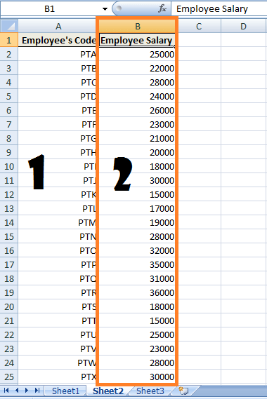
Now consider a workbook with two sheets. Sheet 1 lists Employee Code, Name, and Designation; Sheet 2 lists Employee Code and Employee Salary.
SHEET 1:

SHEET 2:

The objective is to consolidate all data on Sheet 1, as shown below:

VLOOKUP can aggregate data so Employee Code, Name, and Salary appear together in one sheet.
We begin on Sheet 2 because it supplies two arguments — the Employee Salary column is here, and the column index is 2.
We want to find the salary that matches each Employee Code.

The data runs from A2 to B25 — that is our table array.
Step 1) Switch to Sheet 1 and enter the headings shown.

Step 2) Click the cell next to Employee Salary — cell F3 — where the VLOOKUP formula will go.

Enter the VLOOKUP function: =VLOOKUP().
Step 3) Argument 1: Enter F2 — the cell containing the Employee Code to match in the lookup table.

Step 4) Argument 2: The lookup table lives on the other sheet, so reference it with the sheet name: Sheet2!A2:B25.

Step 5) Argument 3: Enter the column index inside the lookup table that holds the return value.
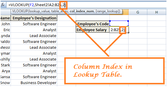

Step 6) Argument 4: Use FALSE for an exact match because we want the exact salary that matches each Employee Code.

Step 7) Press Enter. When you enter an Employee Code, the cell returns the corresponding salary pulled from Sheet 2.

Common VLOOKUP Errors and Fixes
Even experienced users hit VLOOKUP errors. The most common ones, and quick fixes:
- #N/A — VLOOKUP cannot find the lookup value. Check for extra spaces, mismatched data types (numbers stored as text), or that the value really exists in the first column of table_array.
- #REF! — col_index_num is greater than the number of columns in table_array. Lower the column index or extend the range.
- #VALUE! — col_index_num is less than 1 or an argument is invalid. Check the formula syntax.
- Wrong result returned — the fourth argument is TRUE or omitted but the lookup column is unsorted. Switch to FALSE or sort the column ascending.
- Locked references — when copying a formula down, use absolute references (for example, $B$2:$E$25) so the table_array does not drift.
VLOOKUP vs XLOOKUP: Which Should You Use?
Microsoft introduced XLOOKUP in Microsoft 365 and Excel 2021 as a modern replacement for VLOOKUP. It removes several VLOOKUP limitations and is now the recommended choice in supported versions.
| Feature | VLOOKUP | XLOOKUP |
|---|---|---|
| Search direction | Left-to-right only | Any direction (left, right, up, down) |
| Default match type | Approximate (TRUE) | Exact |
| If-not-found handling | Returns #N/A | Built-in if_not_found argument |
| Column index | Hard-coded number | Reference a return-column range |
| Availability | All Excel versions | Microsoft 365, Excel 2021, Excel for the web |
When to choose VLOOKUP: the workbook must run in Excel 2019 or earlier, or you are maintaining legacy formulas. When to choose XLOOKUP: you are building new workbooks in modern Excel and want left lookups, cleaner error handling, and exact match by default. Learn more about lookup functions in the Excel tutorials series.
Conclusion
The three scenarios above explain how VLOOKUP works for exact matches, approximate matches, and cross-sheet references. Practice on your own datasets to build fluency. VLOOKUP remains an important feature in MS-Excel for managing data efficiently, and XLOOKUP extends that toolkit in modern Excel.