
Backpropagation in Neural Network: ML Algorithm & Example
 Editorial Team
⚡ Smart Summary
Backpropagation is the core training algorithm of a neural network, fine-tuning every weight from the error measured in the previous epoch so that the model generalizes better on unseen data, one layer at a time.
What is an Artificial Neural Network?
An artificial neural network is a group of connected I/O units where each connection carries a weight. It helps you to build predictive models from large databases, and the design borrows its vocabulary from the human nervous system. Networks of this kind support image understanding, machine learning, computer speech and many other pattern-recognition tasks.
Backpropagation is the algorithm that decides what those weights should be, so the two ideas are best read together.
What is Backpropagation?
Backpropagation is the essence of neural network training. It is the method of fine-tuning the weights of a neural network based on the error rate obtained in the previous epoch (i.e., iteration). Proper tuning of the weights allows you to reduce error rates and make the model reliable by increasing its generalization.
Backpropagation in neural network is a short form for “backward propagation of errors.” It is a standard method of training artificial neural networks. This method helps calculate the gradient of a loss function with respect to all the weights in the network.
Two terms are often confused. Backpropagation only computes the gradient; an optimizer such as gradient descent is what actually changes the weights using that gradient. Almost every modern framework performs backpropagation automatically through its autodiff engine.
How Backpropagation Algorithm Works
The Back propagation algorithm in neural network computes the gradient of the loss function for a single weight by the chain rule. It efficiently computes one layer at a time, unlike a naive direct computation. It computes the gradient, but it does not define how the gradient is used. It generalizes the computation in the delta rule.
The chain rule is what makes this efficient. The influence of one early weight on the final loss is a product of the local derivatives along the path to the output, so the algorithm caches each layer’s intermediate result on the way back and reuses it for every weight in the layer below instead of recomputing the whole network per weight.
Consider the following Back propagation neural network example diagram to understand. The figure traces one full pass: inputs enter on the left, activations move forward through the hidden layer to the output, and the measured error then travels back along the same connections to correct the weights.
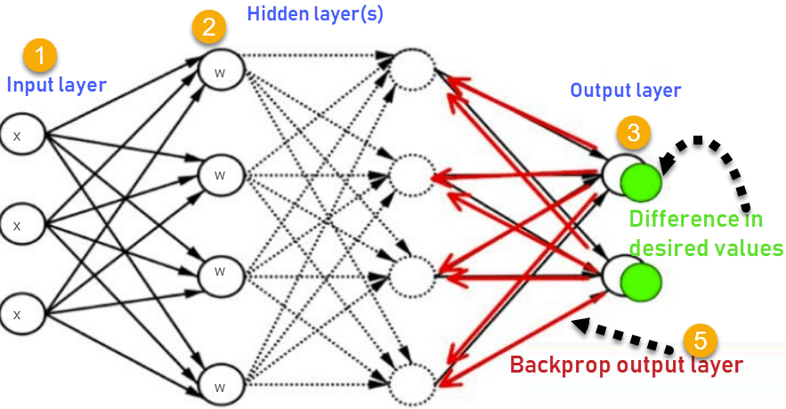
- Inputs X, arrive through the preconnected path
- Input is modeled using real weights W. The weights are usually randomly selected.
- Calculate the output for every neuron from the input layer, to the hidden layers, to the output layer.
- Calculate the error in the outputs:
ErrorB= Actual Output – Desired Output
- Travel back from the output layer to the hidden layer to adjust the weights such that the error is decreased.
- Keep repeating the process until the desired output is achieved.
Many textbooks write the same quantity as desired minus actual. Either convention works, because the sign is absorbed when the optimizer subtracts the gradient, provided you keep one convention throughout the network.
In practice, the error is rarely a bare subtraction. A loss function such as mean squared error for regression, or cross-entropy for classification, converts the per-output differences into the single number whose gradient backpropagation actually computes.
Why We Need Backpropagation?
Most prominent advantages of Backpropagation are:
- Backpropagation is fast, simple and easy to program
- It adds no new parameters of its own; the tuning you do belongs to the optimizer and the network, chiefly the learning rate and the number of inputs
- It is a flexible method as it does not require prior knowledge about the network
- It is a standard method that generally works well
- It does not need any special mention of the features of the function to be learned.
Put simply, without an efficient way to obtain gradients, training anything deeper than a single layer would be computationally impractical.
What is a Feed Forward Network?
A feedforward neural network is an artificial neural network where the nodes never form a cycle. This kind of neural network has an input layer, hidden layers, and an output layer. It is the first and simplest type of artificial neural network.
The distinction matters here because the forward pass of backpropagation is exactly a feedforward pass; only the error correction runs in the opposite direction.
Types of Backpropagation Networks
Two Types of Backpropagation Networks are:
- Static Back-propagation
- Recurrent Backpropagation
Static back-propagation
It is one kind of backpropagation network which produces a mapping of a static input for static output. It is useful to solve static classification issues like optical character recognition.
Recurrent Backpropagation
Recurrent Back propagation in data mining is fed forward until a fixed value is achieved. After that, the error is computed and propagated backward.
The main difference between both of these methods is: that the mapping is rapid in static back-propagation while it is nonstatic in recurrent backpropagation. The table below sets the two side by side.
| Criterion | Static back-propagation | Recurrent backpropagation |
|---|---|---|
| Mapping | Static input to static output | Non-static; the network settles before the error is used |
| Speed | Rapid, one pass per sample | Slower, activation is iterated until it stabilises |
| Network shape | Feedforward, no cycles | Contains feedback connections |
| Typical use | Optical character recognition, fixed-size classification | Problems whose output depends on a settled internal state |
History of Backpropagation
- In 1961, the basic concept of continuous backpropagation was derived in the context of control theory by J. Kelly, Henry Arthur, and E. Bryson.
- In 1969, Bryson and Ho gave a multi-stage dynamic system optimization method.
- In 1970, Seppo Linnainmaa published the reverse mode of automatic differentiation, the computational method that modern backpropagation is built on.
- In 1974, Werbos stated the possibility of applying this principle in an artificial neural network.
- In 1982, Hopfield brought his idea of a neural network.
- In 1986, by the effort of David E. Rumelhart, Geoffrey E. Hinton, Ronald J. Williams, backpropagation gained recognition.
- In 1989, Yann LeCun and colleagues trained a convolutional network with backpropagation to read handwritten digits, one of the first large-scale practical uses.
- In 1993, Wan was the first person to win an international pattern recognition contest with the help of the backpropagation method.
- In 2006, Hinton’s work on deep belief networks and layer-wise pretraining revived interest in training deep networks, which had stalled due to vanishing gradients.
- In 2010, Xavier Glorot and Yoshua Bengio analyzed why deep networks were hard to train and introduced improved weight initialization, which along with ReLU activations made deep backpropagation practical.
- In 2012, AlexNet (Krizhevsky, Sutskever, and Hinton) won the ImageNet competition using GPU-accelerated backpropagation, triggering the modern deep learning boom.
- In 2014, the Adam optimizer (Kingma and Ba) was introduced and quickly became the default gradient-descent variant used with backpropagation.
- In 2015, batch normalization and residual networks (ResNet) solved gradient flow problems in very deep networks, allowing backpropagation through hundreds of layers.
- In 2015-2017, TensorFlow and PyTorch made automatic differentiation a standard software feature, so gradients no longer had to be derived by hand.
- In 2017, the Transformer architecture was introduced, and is trained end-to-end with backpropagation, as are the large language models built on it.
- In 2019, Bengio, Hinton, and LeCun received the ACM A.M. Turing Award for their work on deep neural networks.
- In 2020, the paper “Backpropagation and the Brain” (Lillicrap, Santoro, Marris, Akerman, and Hinton) argued that the brain may approximate backpropagation-like learning, reopening the biological plausibility debate.
- In 2022, Hinton proposed the Forward-Forward algorithm, a training method that avoids a backward pass entirely.
- In 2024, John Hopfield and Geoffrey Hinton were awarded the Nobel Prize in Physics for foundational discoveries that enabled machine learning with artificial neural networks.
- In 2025, forward-forward methods were extended to convolutional networks, showing that backpropagation-free training could work on image classification tasks.
- As of 2026, backpropagation remains the standard training algorithm for virtually all deep learning models, while research continues into gradient-free, local, and parallel learning methods that reduce its memory and compute cost.
Backpropagation Key Points
- Simplifies the network structure by removing weighted links that have the least effect on the trained network
- You need to study a group of input and activation values to develop the relationship between the input and hidden unit layers.
- It helps to assess the impact that a given input variable has on a network output. The knowledge gained from this analysis should be represented in rules.
- Backpropagation is especially useful for deep neural networks working on error-prone projects, such as image or speech recognition.
- Backpropagation takes advantage of the chain and power rules, which allows it to function with any number of outputs.
Best Practice for Backpropagation
Backpropagation in neural network can be explained with the help of the “Shoe Lace” analogy. Weight updates behave much like the tension on a lace: too little and nothing is held together, too much and something snaps.
| Lace tension | What it means during training |
|---|---|
| Too little tension | Not enough constraining and very loose — the model underfits |
| Too much tension | Too much constraint (overtraining); taking too much time (relatively slow process); higher likelihood of breaking |
| Pulling one lace more than the other | Discomfort (bias) — one part of the network dominates the fit |
Two practical habits follow from the analogy: scale the inputs before training so no single feature pulls harder than the rest, and watch the validation loss so the tension is released before overtraining sets in.
Disadvantages of using Backpropagation
- The actual performance of backpropagation on a specific problem is dependent on the input data.
- Back propagation algorithm in data mining can be quite sensitive to noisy data
- Over a mini-batch, backpropagation should be implemented with a matrix-based approach; looping over one example at a time is markedly slower.
- In deep networks the repeated multiplication of small derivatives can shrink gradients towards zero, so the earliest layers barely learn — the vanishing gradient problem described in the Google Machine Learning Crash Course.
None of these rule the method out. They are the reasons practitioners reach for ReLU activations, normalization and careful learning-rate schedules when they move from a shallow network to a deep learning model.
