
Artificial Neural Network (ANN) Tutorial with TensorFlow
 Editorial Team
⚡ Smart Summary
Artificial Neural Networks learn by pushing input through connected layers, scoring the result with a loss function and correcting weights with an optimizer. This walkthrough builds one in TensorFlow and classifies MNIST digits.

What is Artificial Neural Network?
An Artificial Neural Network (ANN) is a computer system inspired by biological neural networks for creating artificial brains based on the collection of connected units called artificial neurons. It is designed to analyse and process information the way humans do. An Artificial Neural Network has self-learning capabilities to produce better results as more data is available.
The diagram below traces one full pass through such a network, from the raw input to the optimizer that corrects the weights.

An Artificial Neural Network (ANN) is composed of four principal objects:
- Layers: all the learning occurs in the layers. There are 3 layers 1) Input 2) Hidden and 3) Output
- Feature and label: Input data to the network (features) and output from the network (labels)
- Loss function: Metric used to estimate the performance of the learning phase
- Optimizer: Improve the learning by updating the knowledge in the network
A neural network takes the input data and pushes it into an ensemble of layers. The network then evaluates its performance with a loss function. The loss function gives the network an idea of the path it needs to take before it masters the knowledge. The network improves that knowledge with the help of an optimizer.
If you take a look at the figure above, you will understand the underlying mechanism.
The program takes some input values and pushes them into two fully connected layers. Imagine you have a math problem. The first thing you do is read the corresponding chapter to solve it. You then apply your new knowledge to the problem. There is a high chance you will not score very well. It is the same for a network: the first time it sees the data and makes a prediction, the result will not match the actual data perfectly.
To improve its knowledge, the network uses an optimizer. In this analogy, an optimizer can be thought of as rereading the chapter. You gain new insights by reading again. Similarly, the network uses the optimizer, updates its knowledge, and tests that new knowledge to check how much it still needs to learn. The program repeats this step until it makes the lowest error possible.
In the math problem analogy, it means you read the textbook chapter many times until you thoroughly understand the course content. Even after reading multiple times, if you keep making an error, it means you reached the knowledge capacity of the current material. You need to use a different textbook or test a different method to improve your score. For a neural network, it is the same process. If the error stops falling and the loss curve goes flat, the current architecture cannot learn anything else. The network has to be better optimized to improve the knowledge.
Those four objects map directly onto the components you configure when you design a network.
Neural Network Architecture
The Artificial Neural Network architecture consists of the following components:
- Layers
- Activation function
- Loss function
- Optimizer
Layers
A layer is where all the learning takes place. Inside a layer sits an arbitrary number of neurons, each holding its own weights. A typical neural network is often processed by densely connected layers (also called fully connected layers). It means all the inputs are connected to the output.
A typical neural network takes a vector of input and a scalar that contains the labels. The simplest setup is a binary classification with only two classes: 0 and 1.
The network takes an input, sends it to all connected nodes and computes the signal with an activation function. The numbered diagram below expands a single node so you can see the weighted sum and the activation step separately.

The figure above plots this idea. The first layer holds the input values. The second layer, called the hidden layer, receives the weighted input from the previous layer.
- The first node is the input values.
- The neuron is decomposed into the input part and the activation function. The left part receives all the input from the previous layer. The right part is the sum of the input passed into an activation function.
- Output value computed from the hidden layers and used to make a prediction. For classification, it is equal to the number of classes. For regression, only one value is predicted.
Activation function
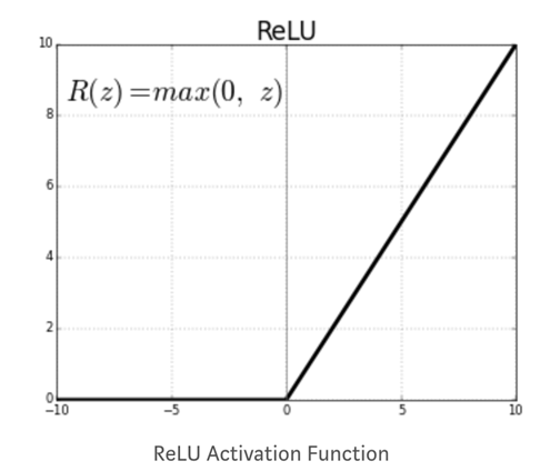
The activation function of a node defines the output given a set of inputs. You need an activation function to allow the network to learn non-linear patterns. A common activation function is ReLU, the Rectified Linear Unit. The function gives a zero for all negative values.
The other activation functions are:
- Piecewise Linear
- Sigmoid
- Tanh
- Leaky ReLU
The plot below shows why ReLU is described that way: the curve is flat at zero for every negative input and rises linearly afterwards.
The critical decision to make when building a neural network is:
- How many layers in the neural network
- How many hidden units for each layer
Neural networks with lots of layers and hidden units can learn a complex representation of the data, but they make the network’s computation very expensive.
Loss function
After you have defined the hidden layers and the activation function, you need to specify the loss function and the optimizer.
For binary classification, it is common practice to use a binary cross entropy loss function. In linear regression, you use the mean square error.
The loss function is an important metric to estimate the performance of the optimizer. During the training, this metric will be minimized. You need to select this quantity carefully depending on the type of problem you are dealing with.
Optimizer
The loss function is a measure of the model’s performance. The optimizer will help improve the weights of the network in order to decrease the loss. There are different optimizers available, but the most common one is Stochastic Gradient Descent.
The conventional optimizers are:
- Momentum optimization
- Nesterov Accelerated Gradient
- AdaGrad
- Adam optimization
Architecture alone does not guarantee a usable model.
Limitations of Neural Network
Following are the limitations of a neural network:
Overfitting
A common problem with a complex neural net is the difficulty of generalizing to unseen data. A neural network with lots of weights can identify specific details in the train set very well, but that often leads to overfitting. If the data are unbalanced within groups (that is, not enough data available in some groups), the network will learn very well during the training but will not have the ability to generalize such patterns to never-seen-before data.
There is a trade-off in machine learning between optimization and generalization.
- Optimizing a model requires finding the best parameters that minimize the loss of the training set.
- Generalization, however, tells how the model behaves for unseen data.
To prevent the model from capturing specific details or unwanted patterns of the training data, you can use different techniques. The best method is to have a balanced dataset with a sufficient amount of data. The art of reducing overfitting is called regularization. The three techniques below are the conventional starting points.
| Technique | What it constrains | Typical setting in this tutorial |
|---|---|---|
| Network size | The number of layers and hidden units | Two hidden layers, 300 and 100 units |
| L1 / L2 weight regularization | The magnitude of the weight coefficients | l1_regularization_strength and l2_regularization_strength of 0.01 |
| Dropout | The share of units switched off per training step | dropout of 0.3 |
Network size
A neural network with too many layers and hidden units is known to be highly sophisticated. A straightforward way to reduce the complexity of the model is to reduce its size. There is no single best practice for defining the number of layers. You need to start with a small number of layers and increase the size until you find the model overfits.
Weight Regularization
A standard technique to prevent overfitting is to add constraints to the weights of the network. The constraint forces the weights of the network to take only small values. The constraint is added to the loss function of the error. There are two kinds of regularization:
- L1 (Lasso): cost is proportional to the absolute value of the weight coefficients.
- L2 (Ridge): cost is proportional to the square of the value of the weight coefficients.
Dropout
Dropout is an odd but useful technique. A network with dropout means that some units will be randomly switched off during a training step, so their outgoing signal becomes zero. Imagine you have an array of weights [0.1, 1.7, 0.7, -0.9]. If the neural network has a dropout, it will become [0.1, 0, 0, -0.9] with randomly distributed 0. The parameter that controls the dropout is the dropout rate. The rate defines how many units are switched off. Having a rate between 0.2 and 0.5 is common.
A small interactive example makes the training loop easy to watch.
Example of Neural Network in TensorFlow
Here is an Artificial Neural Network example in action, showing how a neural network works on a typical classification problem. There are two inputs, x1 and x2, each with a random value. The output is a binary class. The objective is to classify the label based on the two features. To carry out this task, the neural network architecture is defined as follows:
- Two hidden layers
- First layer has four fully connected neurons
- Second layer has two fully connected neurons
- The activation function is a ReLU
- Add an L2 Regularization with a learning rate of 0.003
The network will optimize the weights during 180 epochs with a batch size of 10. In the ANN example animation below, you can see how the weights evolve over time and how the network improves the classification mapping.

First of all, the network assigns random values to all the weights.
- With the random weights, that is, without optimization, the output loss is 0.453. The picture below represents the network with different colors.
- In general, the orange color represents negative values while the blue colors show the positive values.
- The data points have the same representation: the blue ones are the positive labels and the orange ones the negative labels.

Inside the second hidden layer, the lines are colored following the sign of the weights. The orange lines carry negative weights and the blue ones positive weights.
As you can see, in the output mapping, the network is making quite a lot of mistakes. Now look at how the network behaves after optimization.
The picture of the ANN example below depicts the results of the optimized network. First of all, you notice the network has successfully learned how to classify the data points. Comparing it with the picture before, the initial weight was -0.43 while after optimization it results in a weight of -0.95.

The idea can be generalized for networks with more hidden layers and neurons. You can experiment with the settings yourself in the TensorFlow Playground.
The walkthrough below builds the same idea in code against a real dataset.
How to Train a Neural Network with TensorFlow
Here is the step by step process on how to train a neural network with TensorFlow ANN using the API’s estimator DNNClassifier.
We will use the MNIST dataset to train your first neural network. Training a neural network with TensorFlow is not very complicated. The preprocessing step looks precisely the same as in the previous tutorials. You will proceed as follows:
- Import the data
- Transform the data
- Construct the tensor
- Build the model
- Train and evaluate the model
- Improve the model
Version note: the code in this walkthrough targets the TensorFlow 1.x Estimator API. The final release of the tf-estimator package shipped with TensorFlow 2.15, and tf.estimator was removed in TensorFlow 2.16. To run these steps on a current release, either pin TensorFlow 2.15 or rebuild the same two-layer network with tf.keras.layers.Dense and model.fit().
Step 1) Import the data
First of all, you need to import the necessary library. You can import the MNIST dataset using scikit-learn as shown in the TensorFlow Neural Network example below.
The MNIST dataset is the dataset most commonly used to test new techniques or algorithms. It is a collection of 28×28 pixel images, each showing a handwritten digit from 0 to 9. A committee of deep convolutional networks trained with elastic distortions pushed the test error down to 0.27 percent.
import numpy as np
import tensorflow as tf
np.random.seed(1337)
The original walkthrough downloaded the MNIST files by hand and pointed fetch_mldata at that folder.
from sklearn.datasets import fetch_mldata
mnist = fetch_mldata(' /Users/Thomas/Dropbox/Learning/Upwork/tuto_TF/data/mldata/MNIST original')
print(mnist.data.shape)
print(mnist.target.shape)
API note: mldata.org is no longer online and fetch_mldata was removed in scikit-learn 0.22. On a current install, replace the call above with fetch_openml(‘mnist_784’, version=1), which downloads the same 70,000 digits and exposes the identical data and target attributes.
After that, you split the data and get the shape of both datasets.
from sklearn.model_selection import train_test_split

X_train, X_test, y_train, y_test = train_test_split(mnist.data, mnist.target, test_size=0.2, random_state=42)
y_train  = y_train.astype(int)
y_test  = y_test.astype(int)
batch_size =len(X_train)

print(X_train.shape, y_train.shape,y_test.shape )
Step 2) Transform the data
In the previous tutorial, you learned that you need to transform the data to limit the effect of outliers. In this Neural Networks tutorial, you will transform the data using the min-max scaler. The formula is:
(X-min_x)/(max_x - min_x)
scikit-learn already has a function for that: MinMaxScaler()
## resclae
from sklearn.preprocessing import MinMaxScaler
scaler = MinMaxScaler()
# Train
X_train_scaled = scaler.fit_transform(X_train.astype(np.float64))
# test
X_test_scaled = scaler.fit_transform(X_test.astype(np.float64))
Step 3) Construct the tensor
You are now familiar with the way to create tensors in TensorFlow. You can convert the train set to a numeric column.
feature_columns = [tf.feature_column.numeric_column('x', shape=X_train_scaled.shape[1:])]
Step 4) Build the model
The architecture of the neural network contains 2 hidden layers with 300 units for the first layer and 100 units for the second one. These values come from experience rather than from a formula. You can tune them and see how they affect the accuracy of the network.
To build the model, you use the estimator DNNClassifier. You need to set the number of classes to 10 as there are ten classes in the training set. You are already familiar with the syntax of the estimator object. The arguments feature_columns, n_classes and model_dir are precisely the same as in the previous tutorial. The argument hidden_units is the new one: it controls both the number of layers and how many nodes each layer connects to the neural network. In the code below, there are two hidden layers, the first connecting 300 nodes and the second 100 nodes.
To build the estimator, use tf.estimator.DNNClassifier with the following parameters:
- feature_columns: Define the columns to use in the network
- hidden_units: Define the number of hidden neurons
- n_classes: Define the number of classes to predict
- model_dir: Define the path of TensorBoard
estimator = tf.estimator.DNNClassifier(
    feature_columns=feature_columns,
    hidden_units=[300, 100],
    n_classes=10,
    model_dir = '/train/DNN')
Step 5) Train and evaluate the model
You can use the NumPy input function to train the model and evaluate it.
# Train the estimator
train_input = tf.estimator.inputs.numpy_input_fn(
    x={"x": X_train_scaled},
    y=y_train,
    batch_size=50,
    shuffle=False,
    num_epochs=None)
estimator.train(input_fn = train_input,steps=1000)
eval_input = tf.estimator.inputs.numpy_input_fn(
    x={"x": X_test_scaled},
    y=y_test,
    shuffle=False,
    batch_size=X_test_scaled.shape[0],
    num_epochs=1)
estimator.evaluate(eval_input,steps=None)
Output:
{'accuracy': 0.9637143,
 'average_loss': 0.12014342,
 'loss': 1682.0079,
 'global_step': 1000}
The current architecture leads to an accuracy on the evaluation set of roughly 96 percent.
Step 6) Improve the model
You can try to improve the model by adding regularization parameters.
Here the estimator uses a Proximal AdaGrad optimizer with a dropout rate of 0.3 and both L1 and L2 strengths set to 0.01. In a TensorFlow neural network, you reach the optimizer through the train object followed by the name of the optimizer. TensorFlow ships a built-in API for the Proximal AdaGrad optimizer.
To add regularization to the deep neural network, you can use tf.train.ProximalAdagradOptimizer with the following parameters:
- Learning rate: learning_rate
- L1 regularization: l1_regularization_strength
- L2 regularization: l2_regularization_strength
estimator_imp = tf.estimator.DNNClassifier(
    feature_columns=feature_columns,
    hidden_units=[300, 100],
    dropout=0.3,
    n_classes = 10,
    optimizer=tf.train.ProximalAdagradOptimizer(
      learning_rate=0.01,
      l1_regularization_strength=0.01,
      l2_regularization_strength=0.01
    ),
    model_dir = '/train/DNN1')
estimator_imp.train(input_fn = train_input,steps=1000)
estimator_imp.evaluate(eval_input,steps=None)
Output:
{'accuracy': 0.95057142,
 'average_loss': 0.17318928,
 'loss': 2424.6499,
 'global_step': 2000}
The values chosen to reduce the overfitting did not improve the model accuracy. Your first model had an accuracy of 96% while the model with the L2 regularizer has an accuracy of 95%. You can try different values and see how they impact the accuracy.
