
Gaussian Kernel in Machine Learning: Python Kernel Methods
 Editorial Team
⚡ Smart Summary
Gaussian kernel methods make non-separable data linearly separable without ever building the high-dimensional feature map. This walkthrough shows the polynomial mapping by hand, then trains a random Fourier kernel classifier in TensorFlow.
The purpose of this tutorial is to make a dataset linearly separable. The tutorial is divided into two parts:
- Feature transformation
- Train a Kernel classifier with TensorFlow
In the first part, you will understand the idea behind a Kernel method in Machine Learning, while in the second part you will see how to train a kernel classifier with TensorFlow. You will use the adult dataset. The objective of this dataset is to classify the revenue below and above 50k, knowing the behavior of each household.
Why do you need Kernel Methods?
The aim of every classifier is to predict the classes correctly. For that, the dataset should be separable. Look at the plot below; it is fairly simple to see that all points above the black line belong to the first class and the other points to the second class. However, it is extremely rare to have a dataset that simple. In most cases, the data are not separable, and data that is not separable gives naive classifiers like logistic regression a hard time.
import numpy as np
  import matplotlib.pyplot as plt
  from mpl_toolkits.mplot3d import Axes3D
  x_lin = np.array([1,2,3,4,5,6,7,8,9,10])
  y_lin = np.array([2,2,3,2,2,9,6,8,8,9])
  label_lin = np.array([0,0,0,0,0,1,1,1,1,1])

  fig = plt.figure()
  ax=fig.add_subplot(111)
  plt.scatter(x_lin, y_lin, c=label_lin, s=60)
  plt.plot([-2.5, 10], [12.5, -2.5], 'k-', lw=2)
  ax.set_xlim([-5,15])
  ax.set_ylim([-5,15])plt.show()

In the figure below, we plot a dataset which is not linearly separable. If we draw a straight line, most of the points will not be classified in the correct class.
One way to tackle this problem is to take the dataset and transform the data into another feature map. It means you will use a function to move the data to another plane, one that should be linearly separable.
x = np.array([1,1,2,3,3,6,6,6,9,9,10,11,12,13,16,18])
y = np.array([18,13,9,6,15,11,6,3,5,2,10,5,6,1,3,1])
label = np.array([1,1,1,1,0,0,0,1,0,1,0,0,0,1,0,1])
fig = plt.figure()
plt.scatter(x, y, c=label, s=60)
plt.show()
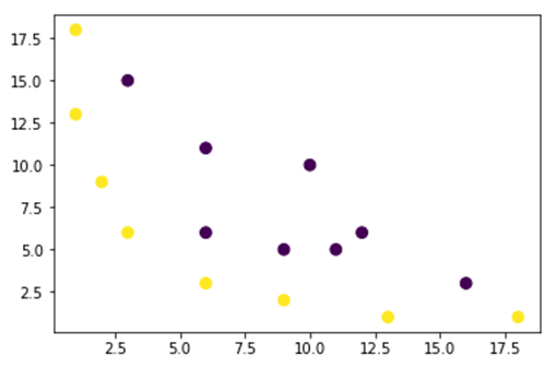
The data from the figure above lies in a 2D plane and is not separable. You can try to transform this data into three dimensions, which means you create a figure with 3 axes.
In our Gaussian Kernel example, we will apply a polynomial mapping to bring our data to a third dimension. The formula to transform the data is as follows.

You define a function in Gaussian Kernel Python to create the new feature maps.
You can use NumPy to code the above formula. Each row below pairs one term of the mapping with the array expression that produces it, and the small image marks the square root of two factor.
| Formula | Equivalent NumPy code |
|---|---|
| x | x[:,0] |
| y | x[:,1] |
| x² | x[:,0]**2 |
 |
np.sqrt(2)* |
| xy | x[:,0]*x[:,1] |
| y² | x[:,1]**2 |
### illustration purpose
def mapping(x, y):
	x = np.c_[(x, y)]
    if len(x) >	2:
    	x_1 = x[:,0]**2
        x_2 = np.sqrt(2)*x[:,0]*x[:,1]
        x_3 = x[:,1]**2
    else:
    	x_1 = x[0]**2
        x_2 = np.sqrt(2)*x[0]*x[1]
        x_3 = x[1]**2
   trans_x = np.array([x_1, x_2, x_3])
   return trans_x
The new mapping has 3 dimensions and 16 points.
x_1  = mapping(x, y)
x_1.shape
(3, 16)
Now make a new plot with 3 axes, x, y and z respectively.
# plot
fig = plt.figure()
ax = fig.add_subplot(111, projection='3d')
ax.scatter(x_1[0], x_1[1], x_1[2], c=label, s=60)
ax.view_init(30, 185)ax.set_xlabel('X Label')
ax.set_ylabel('Y Label')
ax.set_zlabel('Z Label')
plt.show()

We see an improvement, but if we change the orientation of the plot it becomes clear that the dataset is now separable.
# plot
fig = plt.figure()
ax = fig.add_subplot(111, projection='3d')
ax.scatter(x_1[0], x_1[1], x_1[1], c=label, s=60)
ax.view_init(0, -180)ax.set_ylim([150,-50])
ax.set_zlim([-10000,10000])
ax.set_xlabel('X Label')
ax.set_ylabel('Y Label')
ax.set_zlabel('Z Label')plt.show()

If you have to manipulate a large dataset and create more than 2 dimensions, you will face a big problem with the method above. In fact, you need to transform all data points, which is clearly not sustainable. It will take you ages, and your computer may run out of memory.
The most common way to overcome this issue is to use a kernel.
What is a Kernel in machine learning?
The idea is to use a higher-dimension feature space to make the data almost linearly separable, as shown in the figure above.
There are plenty of higher dimensional spaces that make the data points separable. For instance, we have shown that the polynomial mapping is a great start.
We have also demonstrated that with lots of data, these transformations are not efficient. Instead, you can use a Kernel function in Machine Learning to modify the data without moving to a new feature plane.
The magic of the kernel is to find a function that avoids all the trouble implied by the high-dimensional computation. The result of a kernel is a scalar, or said differently, we are back to one-dimensional space.
After you have found this function, you can plug it into the standard linear classifier.
Here is an example that makes the concept of Kernel Machine Learning concrete. You have two vectors, x1 and x2. The objective is to create a higher dimension by using a polynomial mapping. The output is equal to the dot product of the new feature map. From the method above, you need to:
- Transform x1 and x2 into a new dimension
- Compute the dot product: common to all kernels
Transform x1 and x2 into a new dimension
You can use the function created above to compute the higher dimension.
## Kernel
x1 = np.array([3,6])
x2 = np.array([10,10])

x_1 = mapping(x1, x2)
print(x_1)
Output
[[  9.         100.        ]
      [ 25.45584412 141.42135624]
      [ 36.         100.        ]]
Compute the dot product
You can use the object dot from NumPy to compute the dot product between the first and second vector stored in x_1.
print(np.dot(x_1[:,0], x_1[:,1]))
8100.0
The output is 8100. You see the problem: you need to store a new feature map in memory to compute the dot product. If you have a dataset with millions of records, it is computationally ineffective.
Instead, you can use the polynomial kernel to compute the dot product without transforming the vector. This function computes the dot product of x1 and x2 as if these two vectors had been transformed into the higher dimension. Said differently, a kernel function computes the result of the dot product from another feature space.
You can write the polynomial kernel function in Python as follows.
def polynomial_kernel(x, y, p=2):
	return (np.dot(x, y)) ** p
It is the power of the dot product of two vectors. Below, you return the second degree of the polynomial kernel. The output is equal to the other method. This is the magic of the kernel.
polynomial_kernel(x1, x2, p=2)
8100
Types of Kernel Methods
There are lots of different Kernel techniques available. The simplest is the linear kernel. This function works pretty well for text classification. The other kernels are:
- Polynomial kernel
- Gaussian Kernel
The table below summarises what each one does and when practitioners reach for it.
| Kernel | What it computes | Typical use |
|---|---|---|
| Linear | The plain dot product in the original feature space | Already separable data and high-dimensional text features |
| Polynomial | The dot product raised to a degree p, capturing feature interactions | Curved boundaries when the interactions are known to matter |
| Gaussian (RBF) | A distance-based similarity that falls towards zero as points move apart | The usual first choice when the boundary shape is unknown |
In the example with TensorFlow, we will use random Fourier features. TensorFlow has a built-in estimator to compute the new feature space. The random Fourier feature mapper is an approximation of the Gaussian kernel function shown below.

The Gaussian filtering function computes the similarity between the data points in a much higher dimensional space.
With the theory settled, the rest of this walkthrough puts a Gaussian kernel to work on a real dataset.
Train Gaussian Kernel classifier with TensorFlow
The objective of the algorithm is to classify the household earning more or less than 50k.
You will first evaluate a logistic regression to have a benchmark model. After that, you will train a Kernel classifier to see if you can get better results.
You use the following variables from the adult dataset:
- age
- workclass
- fnlwgt
- education
- education_num
- marital
- occupation
- relationship
- race
- sex
- capital_gain
- capital_loss
- hours_week
- native_country
- label
You will proceed as follows before you train and evaluate the model:
- Import the libraries
- Import the data
- Prepare the data
- Construct the logistic model: baseline model
- Evaluate the model
- Construct and evaluate the Kernel classifier
Version note: every snippet below targets TensorFlow 1.x. The tf.contrib namespace, which supplies real_valued_column, RandomFourierFeatureMapper and KernelLinearClassifier, was removed in TensorFlow 2.0, and tf.estimator itself was removed in TensorFlow 2.16. On a current release, build the same pipeline with the tf.keras.layers.experimental.RandomFourierFeatures layer followed by a Dense output layer, or with the RBFSampler and SGDClassifier pair from scikit-learn.
Step 1) Import the libraries
To import and train Kernel models in Artificial Intelligence, you need to import TensorFlow, pandas and NumPy.
#import numpy as np
from sklearn.model_selection
import train_test_split
import tensorflow as tf
import pandas as pd
import numpy as np
Step 2) Import the data
You download the data from the UCI adult dataset page and import it as a pandas DataFrame.
## Define path data
COLUMNS = ['age','workclass', 'fnlwgt', 'education', 'education_num', 'marital', 'occupation', 'relationship', 'race', 'sex', 'capital_gain', 'capital_loss', 'hours_week', 'native_country', 'label']
PATH = "https://archive.ics.uci.edu/ml/machine-learning-databases/adult/adult.data"
PATH_test ="https://archive.ics.uci.edu/ml/machine-learning-databases/adult/adult.test
"## Import
df_train = pd.read_csv(PATH, skipinitialspace=True, names = COLUMNS, index_col=False)
df_test = pd.read_csv(PATH_test,skiprows = 1, skipinitialspace=True, names = COLUMNS, index_col=False)
Now that the train and test set are defined, you can change the column label from string to integer. TensorFlow does not accept string values for the label.
label = {'<=50K': 0,'>50K': 1}
df_train.label = [label[item] for item in df_train.label]
label_t = {'<=50K.': 0,'>50K.': 1}
df_test.label = [label_t[item] for item in df_test.label]
df_train.shape
(32561, 15)
Step 3) Prepare the data
The dataset contains both continuous and categorical features. A good practice is to standardize the values of the continuous variables. You can use the function StandardScaler from scikit-learn. You create a user-defined function as well to make it easier to convert the train and test set. Note that you concatenate the continuous and categorical variables into a common dataset, and the array should be of type float32.
COLUMNS_INT = ['age','fnlwgt','education_num','capital_gain', 'capital_loss', 'hours_week']
CATE_FEATURES = ['workclass', 'education', 'marital', 'occupation', 'relationship', 'race', 'sex', 'native_country']
from sklearn.preprocessing import StandardScaler
from sklearn import preprocessing

def prep_data_str(df):
	scaler = StandardScaler()
    le = preprocessing.LabelEncoder()
    df_toscale = df[COLUMNS_INT]
    df_scaled = scaler.fit_transform(df_toscale.astype(np.float64))
    X_1 = df[CATE_FEATURES].apply(le.fit_transform)
    y = df['label'].astype(np.int32)
    X_conc = np.c_[df_scaled, X_1].astype(np.float32)
    return X_conc, y
The transformer function is ready, so you can convert the dataset and create the input_fn function.
X_train, y_train = prep_data_str(df_train)
X_test, y_test = prep_data_str(df_test)
print(X_train.shape)
(32561, 14)
In the next step, you will train a logistic regression. It will give you a baseline accuracy. The objective is to beat the baseline with a different algorithm, namely a Kernel classifier.
Step 4) Construct the logistic model: Baseline model
You construct the feature column with the object real_valued_column. It will make sure all variables are dense numeric data.
feat_column = tf.contrib.layers.real_valued_column('features', dimension=14)
The estimator is defined using the TensorFlow Estimator API; you supply the feature columns and where to save the graph.
estimator = tf.estimator.LinearClassifier(feature_columns=[feat_column],
                                          n_classes=2,
                                          model_dir = "kernel_log"
                                         )
INFO:tensorflow:Using default config.INFO:tensorflow:Using config: {'_model_dir': 'kernel_log', '_tf_random_seed': None, '_save_summary_steps': 100, '_save_checkpoints_steps': None, '_save_checkpoints_secs': 600, '_session_config': None, '_keep_checkpoint_max': 5, '_keep_checkpoint_every_n_hours': 10000, '_log_step_count_steps': 100, '_train_distribute': None, '_service': None, '_cluster_spec': <tensorflow.python.training.server_lib.ClusterSpec object at 0x1a2003f780>, '_task_type': 'worker', '_task_id': 0, '_global_id_in_cluster': 0, '_master': '', '_evaluation_master': '', '_is_chief': True, '_num_ps_replicas': 0, '_num_worker_replicas': 1}
You will train the logistic regression using mini-batches of size 200.
# Train the model
train_input_fn = tf.estimator.inputs.numpy_input_fn(
	x={"features": X_train},
    y=y_train,
    batch_size=200,
    num_epochs=None,
    shuffle=True)
You can train the model with 1,000 iterations.
estimator.train(input_fn=train_input_fn, steps=1000)
INFO:tensorflow:Calling model_fn.
INFO:tensorflow:Done calling model_fn.
INFO:tensorflow:Create CheckpointSaverHook.
INFO:tensorflow:Graph was finalized.
INFO:tensorflow:Running local_init_op.
INFO:tensorflow:Done running local_init_op.
INFO:tensorflow:Saving checkpoints for 1 into kernel_log/model.ckpt.
INFO:tensorflow:loss = 138.62949, step = 1
INFO:tensorflow:global_step/sec: 324.16
INFO:tensorflow:loss = 87.16762, step = 101 (0.310 sec)
INFO:tensorflow:global_step/sec: 267.092
INFO:tensorflow:loss = 71.53657, step = 201 (0.376 sec)
INFO:tensorflow:global_step/sec: 292.679
INFO:tensorflow:loss = 69.56703, step = 301 (0.340 sec)
INFO:tensorflow:global_step/sec: 225.582
INFO:tensorflow:loss = 74.615875, step = 401 (0.445 sec)
INFO:tensorflow:global_step/sec: 209.975
INFO:tensorflow:loss = 76.49044, step = 501 (0.475 sec)
INFO:tensorflow:global_step/sec: 241.648
INFO:tensorflow:loss = 66.38373, step = 601 (0.419 sec)
INFO:tensorflow:global_step/sec: 305.193
INFO:tensorflow:loss = 87.93341, step = 701 (0.327 sec)
INFO:tensorflow:global_step/sec: 396.295
INFO:tensorflow:loss = 76.61518, step = 801 (0.249 sec)
INFO:tensorflow:global_step/sec: 359.857
INFO:tensorflow:loss = 78.54885, step = 901 (0.277 sec)
INFO:tensorflow:Saving checkpoints for 1000 into kernel_log/model.ckpt.
INFO:tensorflow:Loss for final step: 67.79706.


<tensorflow.python.estimator.canned.linear.LinearClassifier at 0x1a1fa3cbe0>
Step 5) Evaluate the model
You define the NumPy input function to evaluate the model. You use the entire test set for evaluation.
# Evaluation
test_input_fn = tf.estimator.inputs.numpy_input_fn(
    x={"features": X_test},
    y=y_test,
    batch_size=16281,
    num_epochs=1,
    shuffle=False)
estimator.evaluate(input_fn=test_input_fn, steps=1)
INFO:tensorflow:Calling model_fn.
WARNING:tensorflow:Trapezoidal rule is known to produce incorrect PR-AUCs; please switch to "careful_interpolation" instead.
WARNING:tensorflow:Trapezoidal rule is known to produce incorrect PR-AUCs; please switch to "careful_interpolation" instead.
INFO:tensorflow:Done calling model_fn.
INFO:tensorflow:Starting evaluation at 2018-07-12-15:58:22
INFO:tensorflow:Graph was finalized.
INFO:tensorflow:Restoring parameters from kernel_log/model.ckpt-1000
INFO:tensorflow:Running local_init_op.
INFO:tensorflow:Done running local_init_op.
INFO:tensorflow:Evaluation [1/1]
INFO:tensorflow:Finished evaluation at 2018-07-12-15:58:23
INFO:tensorflow:Saving dict for global step 1000: accuracy = 0.82353663, accuracy_baseline = 0.76377374, auc = 0.84898686, auc_precision_recall = 0.67214864, average_loss = 0.3877216, global_step = 1000, label/mean = 0.23622628, loss = 6312.495, precision = 0.7362797, prediction/mean = 0.21208474, recall = 0.39417577
{'accuracy': 0.82353663,
 'accuracy_baseline': 0.76377374,
 'auc': 0.84898686,
 'auc_precision_recall': 0.67214864,
 'average_loss': 0.3877216,
 'global_step': 1000,
 'label/mean': 0.23622628,
 'loss': 6312.495,
 'precision': 0.7362797,
 'prediction/mean': 0.21208474,
 'recall': 0.39417577}
You have an accuracy of 82 percent. In the next section, you will try to beat the logistic classifier with a Kernel classifier.
Step 6) Construct the Kernel classifier
The kernel estimator is not so different from the traditional linear classifier, at least in terms of construction. The idea behind it is to combine the power of an explicit kernel mapping with the linear classifier.
You need two pre-defined estimators available in TensorFlow to train the Kernel Classifier:
- RandomFourierFeatureMapper
- KernelLinearClassifier
You learned in the first section that you need to transform the low dimension into a high dimension using a kernel function. More precisely, you will use random Fourier features, which approximate the Gaussian function. TensorFlow 1.x supplies that mapping as RandomFourierFeatureMapper, and the model can be trained using the estimator KernelLinearClassifier.
To build the model, you will follow these steps:
- Set the high dimension Kernel function
- Set the L2 hyperparameter
- Build the model
- Train the model
- Evaluate the model
Step A) Set the high dimension Kernel function
The current dataset contains 14 features that you will transform into a new 5,000-dimensional vector. You use the random Fourier features to achieve the transformation. If you recall the Gaussian Kernel formula, you note that there is a standard deviation parameter to define. This parameter controls the similarity measure used during the classification: a small stddev makes the kernel treat only very close points as similar, while a large one smooths the decision boundary.
You can tune all the parameters in RandomFourierFeatureMapper with:
- input_dim = 14
- output_dim = 5000
- stddev = 4
### Prep Kernel
kernel_mapper = tf.contrib.kernel_methods.RandomFourierFeatureMapper(input_dim=14, output_dim=5000, stddev=4, name='rffm')
You need to construct the kernel mapper by using the feature columns created before: feat_column
### Map Kernel
kernel_mappers = {feat_column: [kernel_mapper]}
Step B) Set the L2 hyperparameter
To prevent overfitting, you penalize the loss function with the L2 regularizer. You set the L2 hyperparameter to 0.1 and the learning rate to 5.
optimizer = tf.train.FtrlOptimizer(learning_rate=5, l2_regularization_strength=0.1)
Step C) Build the model
The next step is similar to the linear classification. You use the built-in estimator KernelLinearClassifier. Note that you add the kernel mapper defined previously and change the model directory.
### Prep estimator
estimator_kernel = tf.contrib.kernel_methods.KernelLinearClassifier(
    n_classes=2,
    optimizer=optimizer,
    kernel_mappers=kernel_mappers,
    model_dir="kernel_train")
The deprecation warnings below are expected on TensorFlow 1.x, because the kernel_methods module is built on the older tf.contrib.learn estimators.
WARNING:tensorflow:From /Users/Thomas/anaconda3/envs/hello-tf/lib/python3.6/site-packages/tensorflow/contrib/kernel_methods/python/kernel_estimators.py:305: multi_class_head (from tensorflow.contrib.learn.python.learn.estimators.head) is deprecated and will be removed in a future version. Instructions for updating: Please switch to tf.contrib.estimator.*_head. WARNING:tensorflow:From /Users/Thomas/anaconda3/envs/hello-tf/lib/python3.6/site-packages/tensorflow/contrib/learn/python/learn/estimators/estimator.py:1179: BaseEstimator.__init__ (from tensorflow.contrib.learn.python.learn.estimators.estimator) is deprecated and will be removed in a future version. Instructions for updating: Please replace uses of any Estimator from tf.contrib.learn with an Estimator from tf.estimator.* WARNING:tensorflow:From /Users/Thomas/anaconda3/envs/hello-tf/lib/python3.6/site-packages/tensorflow/contrib/learn/python/learn/estimators/estimator.py:427: RunConfig.__init__ (from tensorflow.contrib.learn.python.learn.estimators.run_config) is deprecated and will be removed in a future version. Instructions for updating: When switching to tf.estimator.Estimator, use tf.estimator.RunConfig instead. INFO:tensorflow:Using default config. INFO:tensorflow:Using config: {'_task_type': None, '_task_id': 0, '_cluster_spec': <tensorflow.python.training.server_lib.ClusterSpec object at 0x1a200ae550>, '_master': '', '_num_ps_replicas': 0, '_num_worker_replicas': 0, '_environment': 'local', '_is_chief': True, '_evaluation_master': '', '_train_distribute': None, '_tf_config': gpu_options { per_process_gpu_memory_fraction: 1.0 } , '_tf_random_seed': None, '_save_summary_steps': 100, '_save_checkpoints_secs': 600, '_log_step_count_steps': 100, '_session_config': None, '_save_checkpoints_steps': None, '_keep_checkpoint_max': 5, '_keep_checkpoint_every_n_hours': 10000, '_model_dir': 'kernel_train'}
Step D) Train the model
Now that the Kernel classifier is built, you are ready to train it. You choose to iterate the model 2,000 times.
### estimate
estimator_kernel.fit(input_fn=train_input_fn, steps=2000)
WARNING:tensorflow:Casting <dtype: 'int32'> labels to bool. WARNING:tensorflow:Casting <dtype: 'int32'> labels to bool. WARNING:tensorflow:Trapezoidal rule is known to produce incorrect PR-AUCs; please switch to "careful_interpolation" instead. WARNING:tensorflow:Trapezoidal rule is known to produce incorrect PR-AUCs; please switch to "careful_interpolation" instead. WARNING:tensorflow:From /Users/Thomas/anaconda3/envs/hello-tf/lib/python3.6/site-packages/tensorflow/contrib/learn/python/learn/estimators/head.py:678: ModelFnOps.__new__ (from tensorflow.contrib.learn.python.learn.estimators.model_fn) is deprecated and will be removed in a future version. Instructions for updating: When switching to tf.estimator.Estimator, use tf.estimator.EstimatorSpec. You can use the `estimator_spec` method to create an equivalent one. INFO:tensorflow:Create CheckpointSaverHook. INFO:tensorflow:Graph was finalized. INFO:tensorflow:Running local_init_op. INFO:tensorflow:Done running local_init_op. INFO:tensorflow:Saving checkpoints for 1 into kernel_train/model.ckpt. INFO:tensorflow:loss = 0.6931474, step = 1 INFO:tensorflow:global_step/sec: 86.6365 INFO:tensorflow:loss = 0.39374447, step = 101 (1.155 sec) INFO:tensorflow:global_step/sec: 80.1986 INFO:tensorflow:loss = 0.3797774, step = 201 (1.247 sec) INFO:tensorflow:global_step/sec: 79.6376 INFO:tensorflow:loss = 0.3908726, step = 301 (1.256 sec) INFO:tensorflow:global_step/sec: 95.8442 INFO:tensorflow:loss = 0.41890752, step = 401 (1.043 sec) INFO:tensorflow:global_step/sec: 93.7799 INFO:tensorflow:loss = 0.35700393, step = 501 (1.066 sec) INFO:tensorflow:global_step/sec: 94.7071 INFO:tensorflow:loss = 0.35535482, step = 601 (1.056 sec) INFO:tensorflow:global_step/sec: 90.7402 INFO:tensorflow:loss = 0.3692882, step = 701 (1.102 sec) INFO:tensorflow:global_step/sec: 94.4924 INFO:tensorflow:loss = 0.34746957, step = 801 (1.058 sec) INFO:tensorflow:global_step/sec: 95.3472 INFO:tensorflow:loss = 0.33655524, step = 901 (1.049 sec) INFO:tensorflow:global_step/sec: 97.2928 INFO:tensorflow:loss = 0.35966292, step = 1001 (1.028 sec) INFO:tensorflow:global_step/sec: 85.6761 INFO:tensorflow:loss = 0.31254214, step = 1101 (1.167 sec) INFO:tensorflow:global_step/sec: 91.4194 INFO:tensorflow:loss = 0.33247527, step = 1201 (1.094 sec) INFO:tensorflow:global_step/sec: 82.5954 INFO:tensorflow:loss = 0.29305756, step = 1301 (1.211 sec) INFO:tensorflow:global_step/sec: 89.8748 INFO:tensorflow:loss = 0.37943482, step = 1401 (1.113 sec) INFO:tensorflow:global_step/sec: 76.9761 INFO:tensorflow:loss = 0.34204718, step = 1501 (1.300 sec) INFO:tensorflow:global_step/sec: 73.7192 INFO:tensorflow:loss = 0.34614792, step = 1601 (1.356 sec) INFO:tensorflow:global_step/sec: 83.0573 INFO:tensorflow:loss = 0.38911164, step = 1701 (1.204 sec) INFO:tensorflow:global_step/sec: 71.7029 INFO:tensorflow:loss = 0.35255936, step = 1801 (1.394 sec) INFO:tensorflow:global_step/sec: 73.2663 INFO:tensorflow:loss = 0.31130585, step = 1901 (1.365 sec) INFO:tensorflow:Saving checkpoints for 2000 into kernel_train/model.ckpt. INFO:tensorflow:Loss for final step: 0.37795097. KernelLinearClassifier(params={'head': <tensorflow.contrib.learn.python.learn.estimators.head._BinaryLogisticHead object at 0x1a2054cd30>, 'feature_columns': {_RealValuedColumn(column_name='features_MAPPED', dimension=5000, default_value=None, dtype=tf.float32, normalizer=None)}, 'optimizer': <tensorflow.python.training.ftrl.FtrlOptimizer object at 0x1a200aec18>, 'kernel_mappers': {_RealValuedColumn(column_name='features', dimension=14, default_value=None, dtype=tf.float32, normalizer=None): [<tensorflow.contrib.kernel_methods.python.mappers.random_fourier_features.RandomFourierFeatureMapper object at 0x1a200ae400>]}})
Step E) Evaluate the model
Last but not least, you evaluate the performance of your model. You should be able to beat the logistic regression.
# Evaluate and report metrics.
eval_metrics = estimator_kernel.evaluate(input_fn=test_input_fn, steps=1)
WARNING:tensorflow:Casting <dtype: 'int32'> labels to bool. WARNING:tensorflow:Casting <dtype: 'int32'> labels to bool. WARNING:tensorflow:Trapezoidal rule is known to produce incorrect PR-AUCs; please switch to "careful_interpolation" instead. WARNING:tensorflow:Trapezoidal rule is known to produce incorrect PR-AUCs; please switch to "careful_interpolation" instead. INFO:tensorflow:Starting evaluation at 2018-07-12-15:58:50 INFO:tensorflow:Graph was finalized. INFO:tensorflow:Restoring parameters from kernel_train/model.ckpt-2000 INFO:tensorflow:Running local_init_op. INFO:tensorflow:Done running local_init_op. INFO:tensorflow:Evaluation [1/1] INFO:tensorflow:Finished evaluation at 2018-07-12-15:58:51 INFO:tensorflow:Saving dict for global step 2000: accuracy = 0.83975184, accuracy/baseline_label_mean = 0.23622628, accuracy/threshold_0.500000_mean = 0.83975184, auc = 0.8904007, auc_precision_recall = 0.72722375, global_step = 2000, labels/actual_label_mean = 0.23622628, labels/prediction_mean = 0.23786618, loss = 0.34277728, precision/positive_threshold_0.500000_mean = 0.73001117, recall/positive_threshold_0.500000_mean = 0.5104004
The final accuracy is 84%, about 1.6 percentage points above the logistic regression baseline (0.83975184 against 0.82353663). There is a tradeoff between accuracy improvement and computational cost. You need to think about whether that improvement is worth the time consumed by the heavier classifier and whether it has a compelling impact on your business.
