SAP HANA Calculation View Tutorial

What is Calculation View?

SAP HANA Calculation view is a powerful information view.

SAP HANA Analytic view measure can be selected from only one fact table. When there is need of More Fact table in information view then calculation view come in the picture. Calculation view supports complex calculation.

The data foundation of the calculation view can include tables, column views, analytic views and calculation views.

We can create Joins, Unions, Aggregation, and Projections on data sources.

Calculation View can contain multiple measures and can be used for multidimensional reporting or no measure which is used in list type reporting.

Characteristic of SAP HANA Calculation View as below –

• Support Complex Calculation.
• Support OLTP and OLAP models.
• Support Client handling, language, currency conversion.
• Support Union, Projection, Aggregation, Rank, etc.

SAP HANA Calculation View are of two types –

1. SAP HANA Graphical Calculation View (Created by SAP HANA Studio Graphical editor).
2. SAP HANA Script-based calculations Views (Created by SQL Scripts by SAP HANA Studio).

SAP HANA Graphical Calculation View

In SAP HANA Analytic view, we can select a measure from one table only.

So when there is a requirement for a view which contains measure from the different table then it cannot achieve by analytic view but by calculation view.

So in this case, we can use two different analytic view for each table and join them in calculation view.

We are going to create a graphical Calculation View “CA_FI_LEDGER” by joining two Analytic View “AN_PURCHASE_ORDER” And “AN_FI_DOCUMENT”.

CA_FI_LEDGER will display finance document detail related to a purchase order.

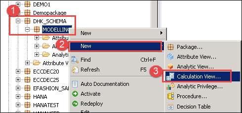
Step 1) In this step,

1. Go to package (Here Modelling) and right click.
2. Select New Option.
3. Select Calculation View.

A Calculation View Editor will be displayed, in which Scenario Panel display as below –

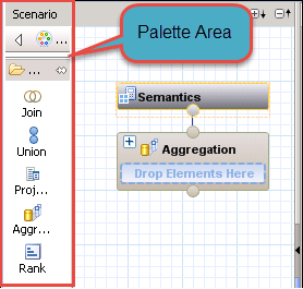
Detail of Scenario panel is as below –

• Palette: This section contains below nodes that can be used as a source to build our calculation views.

We have 5 different types of nodes, they are

1. Join: This node is used to join two source objects and pass the result to the next node. The join types can be inner, left outer, right outer and text join.Note: We can only add two source objects to a join node.
2. Union: This is used to perform union all operation between multiple sources. The source can be n number of objects.
3. Projection: This is used to select columns, filter the data and create additional columns before we use it in next nodes like a union, aggregation and rank.Note: We can only add one source objects in a Projection node.
4. Aggregation: This is used to perform aggregation on specific columns based on the selected attributes.
5. Rank: This is the exact replacement for RANK function in SQL. We can define the partition and order by clause based on the requirement.

Step 2)

1. Click Projection node from palette and drag and drop to scenario area from Purchase order analytic view. Renamed it to “Projection_PO”.
2. Click Projection node from palette and drag and drop to scenario area for FI Document analytic view. Renamed it to “Projection_FI”.
3. Drag and drop analytic View “AN_PUCHASE_ORDER” “AN_FI_DOCUMENT” and from Content folder to Projection node and “Projection_FI” respectively.
4. Click Join Node from Palette and drag and drop to scenario area.
5. Join Projection_PO node to Join_1 node.
6. Join Projection_FI node to Join_1 node.
7. Click Aggregation node from palette and drag and drop to scenario area.
8. Join Join_1 node to Aggregation node.

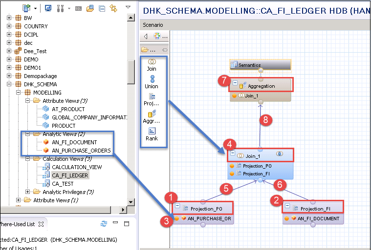
We have added two analytic views, for creating a calculation view.

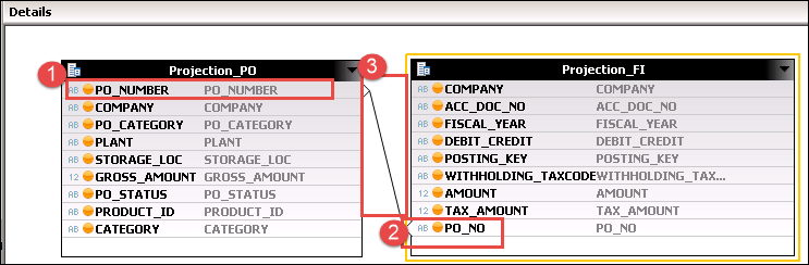
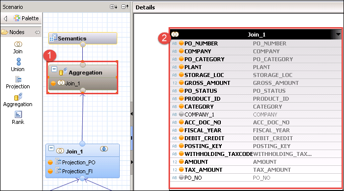
Step 3) Click on Join_1 node under aggregation and you can see the detail section is displayed.

1. Select all column from Projection_PO Node for output.
2. Select all column from Projection_FI node for output.
3. Join Projection_PO Node to Projection_FI node on columnProjection_PO. PO_Number = Projection_FI.PO_NO.

Step 4) In this step,

1. Click on Aggregation node and Detail will be displayed on right side of the pane.
2. Select Column for output from the Join_1 displayed on the right side in the detail window.

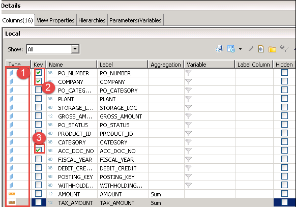
Step 5) Now, click on Semantics Node.

Detail screen will be displayed as below. Define attribute and measure type for the column and also, mark key for this output.

1. Define attribute and measure.
2. Mark PO_Number and COMPANY as Key.
3. Mark ACC_DOC_NO as key.

Step 6) Validate and Activate calculation View, from the top bar of the window.

1. Click on Validate Icon.
2. Click on Activate Icon.

Calculation View will be activated and will display under Modelling Package as below –

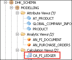
Select calculation view and right click ->Data preview

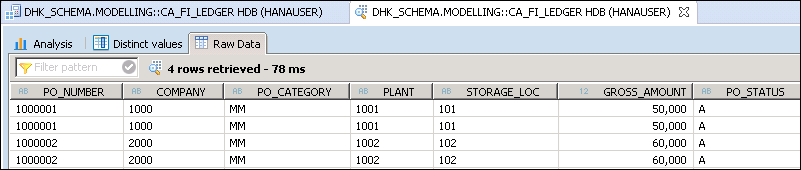
We have added two analytic views and select measure (TAX_AMOUNT, GROSS_AMOUNT) from both analytic view.

Data Preview screen will be displayed as below –

CE Functions also known as Calculation Engine Plan Operator (CE Operators) are alternative to SQL Statements.

CE function is two types –

Data Source Access Function

This function binds a column table or a column view to a table variable.

Below is some data Source Access Function list –

• CE_COLUMN_TABLE
• CE_JOIN_VIEW
• CE_OLAP_VIEW
• CE_CALC_VIEW

Relational Operator Function

By Using Relational Operator, the user can bypass the SQL processor during the evaluation and communicate with calculation engine directly.

Below is some Relational Operator Function list –

• CE_JOIN (It is used to perform inner join between two sources and Read the required columns/data.)
• CE_RIGHT_OUTER_JOIN(It is used to perform right outer join between the two sources and display the queried columns to the output.)
• CE_LEFT_OUTER_JOIN (It is used to perform left outer join between the sources and display the queried columns to the output).
• CE_PROJECTION (This function display the specific columns from the source and apply filters to restrict the data. It provides column name aliase features also.)
• CE_CALC (It is used to calculate additional columns based on the business requirement. This is same as calculated column in graphical models.)

Below is a list of SQL with CE function with some Example-

Query Name	SQL Query	CE-Build in Function
Select Query On Column Table	SELECT C, D From “COLUMN_TABLE”.	CE_COLUMN_TABLE(“COLUMN_TABLE”,[C,D])
Select Query On Attribute View	SELECT C, D From “ATTRIBUTE_VIEW”	CE_JOIN_VIEW(“ATTRIBUTE_VIEW”,[C,D])
Select Query on Analytic View	SELECT C, D, SUM(E) From “ANALYTIC_VIEW” Group By C,D	CE_OLAP_VIEW(“ANALYTIC_VIEW”,[C,D])
Select Query on Calculation View	SELECT C, D, SUM(E) From “CALCULATION_VIEW” Group By C,D	CE_CALC_VIEW(“CALCULATION_VIEW”,[C,D])
Where Having	SELECT C, D, SUM(E) From “ANALYTIC_VIEW” Where C = ‘value’	Var1= CE_COLUMN_TABLE(“COLUMN_TABLE”); CE_PROJECTION(:var1,[C,D],”C” =”value”/