SAP HANA Analytic View: How to Create & Use

What is an Analytic View in SAP HANA?

An analytic view in SAP HANA is based on star schema modeling and represents an OLAP, or multidimensional, modeling object. It forms a cube-like structure that is used to analyze data, and it suits any scenario where aggregated data from the underlying tables is needed.

In an analytic view, dimension tables are joined to the fact table that holds the transaction data. A dimension table carries descriptive data such as product, product name, vendor or customer. A fact table carries descriptive data together with measurable data such as amount and tax.

Because the aggregation happens in memory at query time, no aggregate tables have to be stored. The view is defined once in SAP HANA modeling and reused by every report that reads it.

Example of SAP HANA Analytic View

Here, an analytic view is created for a purchase order, based on the attribute view “AT_PRODUCT” created earlier. The Purchase Order Header table and the Purchase Order Detail table supply the transaction data.

Run both scripts below in the SQL console of SAP HANA Studio before the modeling steps begin.

SQL script to create table “PURCHASE_ORDER” in “DHK_SCHEMA”

CREATE COLUMN TABLE "DHK_SCHEMA"."PURCHASE_ORDER"					
(		
PO_NUMBER NVARCHAR(10) primary key,							
COMPANY NVARCHAR (4),			
PO_CATEGORY NVARCHAR(2),			
PRODUCT_ID NVARCHAR(10),			
VENDOR NVARCHAR(10),			
TERMS NVARCHAR(4),			
PUR_ORG NVARCHAR(4),			
PUR_GRP NVARCHAR(3),			
CURRENCY NVARCHAR(5),			
QUOTATION_NO NVARCHAR(10),			
PO_STATUS VARCHAR(1),			
CREATED_BY NVARCHAR(20),			
CREATED_AT DATE		
);		

INSERT	INTO "DHK_SCHEMA"."PURCHASE_ORDER" VALUES(1000001,1000,'MM','A0001','V000001','CASH' ,1000,'GR1','INR',1000011,'A','HANAUSER','2016-01-07');																													
INSERT INTO "DHK_SCHEMA"."PURCHASE_ORDER" VALUES(1000002,2000,'MM','A0002','V000001','CASH',1000,'GR1','INR',1000012,'A','HANAUSER','2016-01-06');																			
INSERT INTO "DHK_SCHEMA"."PURCHASE_ORDER" VALUES(1000003,2000,'MM','A0003','V000001','CASH',1000,'GR1','INR',1000013,'A','HANAUSER','2016-01-07');																			
INSERT INTO "DHK_SCHEMA"."PURCHASE_ORDER" VALUES(1000004,2000,'MM','A0004','V000001','CASH',1000,'GR1','INR',1000014,'A','HANAUSER','2016-01-07');

SQL script to create table “PURCHASE_DETAIL” in “DHK_SCHEMA”

CREATE	 COLUMN TABLE "DHK_SCHEMA"."PURCHASE_DETAIL"					
(		
PO_NUMBER NVARCHAR(10) primary key,							
COMPANY NVARCHAR(4),			
PO_CATEGORY NVARCHAR(2),			
PRODUCT_ID NVARCHAR(10),			
PLANT NVARCHAR(4),			
STORAGE_LOC NVARCHAR(4),			
VENDOR NVARCHAR(10),			
TERMS NVARCHAR(4),			
PUR_ORG NVARCHAR(4),			
PUR_GRP NVARCHAR(3),			
CURRENCY NVARCHAR(5),			
QUANTITY SMALLINT,			
QUANTITY_UNIT VARCHAR(4),			
ORDER_PRICE DECIMAL(8,2),			
NET_AMOUNT DECIMAL(8,2),			
GROSS_AMOUNT DECIMAL(8,2),			
TAX_AMOUNT DECIMAL(8,2)			
);		


INSERT	INTO "DHK_SCHEMA"."PURCHASE_DETAIL"	VALUES(1000001,1000,'MM','A0001',1001,101,
'V000001','CASH',1000,'GR1','INR',10,'UNIT',50000.00,40000.00,50000.00,10000.00);																									
INSERT	INTO "DHK_SCHEMA"."PURCHASE_DETAIL"	VALUES(1000002,2000,'MM','A0002',1002,102,
'V000002','CASH',1000,'GR1','INR',10,'UNIT',60000.00,48000.00,60000.00,12000.00);																									
INSERT	INTO "DHK_SCHEMA"."PURCHASE_DETAIL"	VALUES(1000003,2000,'MM','A0003',1003,103,
'V000001','CASH',1000,'GR1','INR',20,'UNIT',40000.00,32000.00,40000.00,8000.00);																									
INSERT	INTO "DHK_SCHEMA"."PURCHASE_DETAIL"	VALUES(1000004,2000,'MM','A0004',1004,104,
'V000002','CASH',1000,'GR1','INR',20,'UNIT',20000.00,16000.00,20000.00,4000.00);																	

The two scripts create the tables “PURCHASE_ORDER” and “PURCHASE_DETAIL” together with their data.

How to Create an Analytic View in SAP HANA

An analytic view named “AN_PURCHASE_ORDERS” is created below from the attribute view “AT_PRODUCT” and the tables “PURCHASE_ORDER” and “PURCHASE_DETAIL”. The ten steps follow the order of the editor screens.

Step 1) Create a new analytic view from the package tree shown below.

1. Select the Modelling sub-package under the DHK_SCHEMA package.
2. Right-click and choose New.
3. Select the Analytic View option.

Step 2) The information view editor opens for the analytic view. Complete the creation dialog shown below.

1. Enter the analytic view name “AN_PURCHASE_ORDERS” and a label for it.
2. Select the view type “Analytic View”.

Once the entries are complete, click the Finish button. The information view editor is then displayed for the analytic view.

Step 3) Add the tables from the schema to the Data Foundation node under the scenario pane. The scenario pane holds three nodes.

1. Semantics: this node represents the output structure of the view.
2. Star Join: this node creates the join that attaches the attribute views to the fact table.
3. Data Foundation: this node holds the fact tables of the analytic view. Several tables can be added, but measures can be selected from only one of them.

Drag and drop the tables “PURCHASE_ORDER” and “PURCHASE_DETAIL” from DHK_SCHEMA onto the Data Foundation node, as shown below.

Step 4) Add the attribute view to the Star Join node.

1. Select the “AT_PRODUCT” attribute view from the Modelling package.
2. Drag and drop the attribute view onto the Star Join node, as shown below.

Step 5) In the same window, work in the detail panel as directed.

1. Click the Data Foundation node. The tables added to it appear in the detail section.
2. Join the table “PURCHASE_ORDER” to the table “PURCHASE_DETAIL” on the “PO_NUMBER” field.
3. Enter the join type and the cardinality.

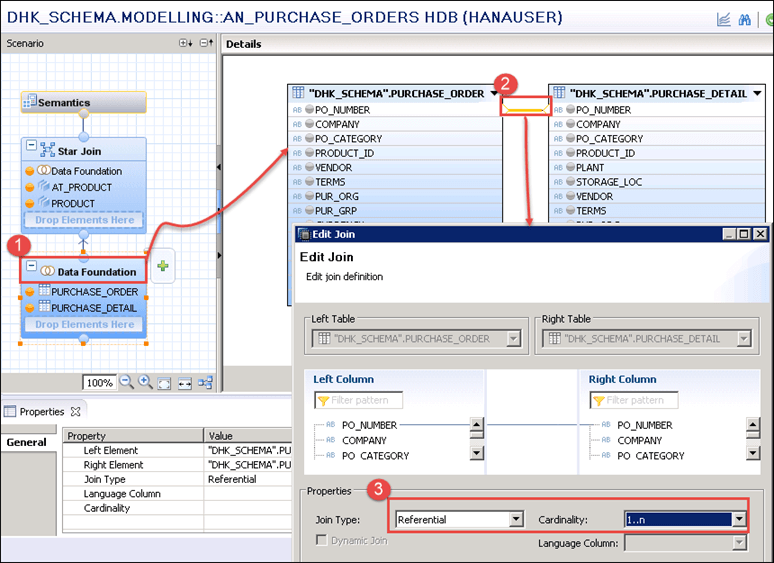
Click the OK button to keep the join.

Step 6) Select the following columns in the same window.

1. Select PO_NUMBER, COMPANY, PO_CATEGORY, PRODUCT_ID, PLANT and STORAGE_LOC from the “PURCHASE_DETAIL” table.
2. Select the CURRENCY column from the “PURCHASE_DETAIL” table.
3. Select GROSS_AMOUNT and TAX_AMOUNT.
4. Select the PO_STATUS, CREATED_BY and CREATED_AT columns from the “PURCHASE_ORDER” table, which is the purchase order header.

Every selected column, marked in orange, appears in the output of the analytic view.

Step 7) Join the attribute view to the fact table in the data foundation. Click the Star Join node in the scenario pane, as shown below.

The attribute view and the fact table are displayed in the detail pane. Join the attribute view to the data foundation on the “PRODUCT_ID” column, as shown below.

Click the join link. A pop-up for Edit Join is displayed, where the join type is defined as “Referential” and the cardinality as 1…1.

Click the OK button to confirm the star join.

Step 8) Define the attributes, the measures and the key of the view. Select the Semantics node in the scenario pane, as shown below.

1. Select the Columns tab in the detail pane.
2. Define the column type as attribute or measure. Every column here is an attribute except “GROSS_AMOUNT”, which is defined as a measure.

Step 9) Validate and activate the analytic view from the toolbar.

1. Validate the analytic view.
2. Activate the analytic view.

The analytic view “AN_PURCHASE_ORDERS” is now created and activated in the Analytic folder of the Modelling sub-package, as shown below.

Step 10) Preview the data in the analytic view.

1. Go to the toolbar section and click the “Data Preview” icon.
2. Select Open in Data Preview Editor.

Three tabs are available in the data preview editor. The Analysis tab takes attributes and measures by drag and drop into the label axis and the value axis, and shows the output as a chart, table, grid or HTML, as below.

The Distinct values tab shows the distinct values of one selected attribute at a time, as below.

The Raw Data tab shows the records in table format, as below.

Note: an analytic view accepts only attribute views as its dimensions and does not support the union operator. Row-level restrictions on the activated view are applied through analytic privileges.

Attribute views and analytic views are deprecated as of SAP HANA 2.0 and are not available in SAP HANA Cloud, so new cube-style models are built as graphical calculation views of data category Cube with star join. The steps above still apply to existing SAP HANA 2.0 systems, and the modeling concepts carry over. More background is available in the SAP HANA series.

FAQs