SAP DS (Data Services) in HANA

What is SAP Data Services?

SAP Data Services is an ETL tool which gives a single enterprise level solution for data integration, transformation, data quality, data profiling, and text data processing from a heterogeneous source into a target database or data warehouse.

Applications, called jobs, are created in the Designer, where data mapping and transformation are defined. The product is also referred to as SAP BusinessObjects Data Services, abbreviated to SAP BODS, and both names describe the same tool. SAP Data Services 4.3 is the current release; version 4.2 reached end of mainstream maintenance on 31 May 2023, so new implementations should start on 4.3.

Within an SAP HANA landscape, SAP Data Services is the option chosen when data needs to be reshaped on the way in rather than copied as it stands. The sections below cover what the tool offers, how its parts fit together, and a complete worked load from an SAP ECC table into SAP HANA.

Features of SAP Data Services

The capabilities below explain why SAP Data Services is positioned as an enterprise grade platform rather than a simple copy utility.

• It provides high-performance parallel transformations.
• It has comprehensive administrative tools and a reporting tool.
• It supports multiple users.
• SAP BODS is very flexible with web-service based applications.
• It allows a scripting language with rich sets of functions.
• SAP Data Services can integrate with SAP LT Replication Server (SLT) using trigger-based technology. SLT adds delta capabilities to every SAP or non-SAP source table, which allows change data capture and the transfer of delta data from the source table.
• Data validation with dashboards and process auditing.
• An administration tool with scheduling capabilities and monitoring dashboards.
• Debugging, built-in profiling, and data viewing.
• SAP Data Services supports a broad range of sources and targets:
• Any application, for example SAP.
• Any database, with bulk loading and change data capture.
• Files: fixed width, comma delimited, COBOL, XML, and Excel.

These features are delivered by a small set of installable components, each with a distinct role.

Components of SAP Data Services

SAP Data Services has the components below.

1. Designer – It is a development tool by which we can create, test, and execute a job that populates a data warehouse. It allows the developer to create objects and configure them by selecting an icon in a source-to-target flow diagram. It can be used to create an application by specifying workflows and data flows. To open Data Services Designer, go to Start Menu -> All Programs -> SAP Data Services -> Data Services Designer.

2. Job Server – It is an application that launches the Data Services processing engine and serves as an interface to the engine and the Data Services suite.
3. Engine – The Data Services engine executes the individual jobs which are defined in the application.
4. Repository – The repository is a database that stores Designer predefined objects and user defined objects (source and target metadata, transformation rules). Repositories are of two types:

• Local Repository (used by Designer and Job Server).
• Central Repository (used for object sharing and version control).

5. Access Server – The Access Server passes messages between web applications, the Data Services Job Server, and the engines.
6. Administrator – The web Administrator provides browser-based administration of Data Services resources, detailed as below:

• Configuring, starting, and stopping real-time services.
• Scheduling, monitoring, and executing batch jobs.
• Configuring Job Server, Access Server, and repository usage.
• Managing users.
• Publishing batch jobs and real-time services through web services.
• Configuring and managing adapters.

Knowing what each component does is only half the picture. The architecture below shows how they communicate during a load.

SAP Data Services Architecture

The Data Services architecture has the following components:

• Central Repository – it is used for repository configurations to Job Servers, security management, version control, and object sharing.
• Designer – used to create a project, job, workflow, and data flow, and to run them.
• Local Repository – here you can create, change, and start jobs, workflows, and data flows.
• Job Server & Engine – it manages the jobs.
• Access Server – it is used to execute the real-time jobs created by developers in the repositories.

In the image below, Data Services and the relationships between its components are shown.

SAP BODS Architecture

Designer Window Detail

The Designer is the component a developer spends the most time in, so its layout is worth learning first. The detail of each section of the Data Services Designer is as below:

1. Tool Bar (used for Open, Save, Back, Validate, Execute, etc.).
2. Project Area (contains the current project, which includes job, workflow, and data flow. In Data Services, all entities are objects).
3. Work Space (the application window area in which we define, display, and modify objects).
4. Local Object Library (it contains local repository objects, such as transforms, job, workflow, data flow, etc.).
5. Tool Palette (buttons on the tool palette enable you to add new objects to the workspace).

Object Hierarchy

The diagram below shows the hierarchical relationships for the key object types within Data Services.

Note: the legend below identifies the optional elements in the hierarchy.

Workflows and conditionals are optional.

The objects used in SAP Data Services are detailed below.

Objects	Description
Project	A project is the highest-level object in the Designer window. Projects provide you with a way to organize the other objects you create in Data Services. Only one project is open at a time, where “open” means “visible in the project area”.
Job	A “job” is the smallest unit of work that you can schedule independently for execution.
Scripts	A subset of lines in a procedure.
Workflow	A “workflow” is the incorporation of several data flows into a coherent flow of work for an entire job. A workflow is optional. A workflow is a procedure that can: Call data flows Call another workflow Define the order of steps to be executed in your job Pass parameters to and from data flows Specify how to handle errors that occur during execution Define conditions for executing sections of the project
Dataflow	A “data flow” is the process by which source data is transformed into target data. A data flow is a reusable object. It is always called from a workflow or a job. It is used to: Identify the source data that you want to read Define the transformations that you want to perform on the data Identify the target table to which you want to load data
Datastore	A logical channel that connects Data Services to source and target databases. Datastores: Must be specified for each source and target database Are used to import metadata for source and target databases into the repository Are used by Data Services to read data from source tables and load data to target tables
Target	The table or file into which Data Services loads data from the source.

SAP Data Services vs SLT vs DXC

SAP Data Services is one of several data provisioning options for SAP HANA, and choosing the wrong one adds cost that no amount of tuning recovers. The table below compares the three server-side methods.

Criteria	SAP Data Services	SLT	DXC
Latency	Batch or scheduled	Real time	Batch, scheduled by DataSource
Transformation	Full ETL, cleansing and profiling	Simple filter and field rules	None beyond extractor logic
Source scope	SAP and non-SAP, files, applications	SAP and non-SAP databases	SAP Business Suite only
Extra server required	Yes, Job Server	Usually yes	No
Best suited to	Data quality and multi-source consolidation	Operational reporting on live data	Reusing existing Business Content extractors

In short, choose SAP Data Services when data must be cleansed, joined, or standardised before it lands. Choose SLT when the report has to reflect the transaction as it happens, and DXC when a proven Business Content extractor already produces the semantics you need. For a one-off dataset with no repeat schedule, a flat file upload is faster than configuring any of the three.

How to Load Data from an SAP Source Table Using SAP Data Services

Everything in Data Services is an object. A separate datastore is needed for each source and target database.

The full sequence for loading data from an SAP source table is listed below. Each step is then shown in detail.

• Create a datastore between the source and BODS
• Import the metadata (structures) into BODS
• Configure the Import Server
• Import the metadata into the HANA system
• Create a datastore between BODS and HANA
• Create a project
• Create a job (batch or real time)
• Create a workflow
• Create a data flow
• Add objects to the data flow
• Execute the job
• Check the data preview in HANA

Step 1) Create a datastore between the SAP source and BODS.

1. To load data from an SAP source into SAP HANA through SAP BODS, a datastore is required. So we create a datastore first, as shown below – Project -> New -> Data Store

2. A pop-up for Create New Datastore will appear. Enter the details as below:
   1. Enter the datastore name “ds_ecc”.
   2. Select the datastore type name as “SAP Applications”.
   3. Enter the database server name.
   4. Enter the user name and password.
   5. Click on the “Apply” button.
   6. Click on the “OK” button.

3. The datastore will be created. View the created datastore as below.

1. Go to the Local Object Library.
2. Select the Datastore tab.
3. The datastore “ds_ecc” will be displayed.

Step 2) Import metadata (structure) into the BODS server.

We have created a datastore for ECC to BODS; now we import metadata from ECC into BODS. To import, follow the steps below.

1. Select the datastore “ds_ecc” and right-click.
2. Select the Import by Name option.

A pop-up for Import by Name will be displayed. Enter the details as below:

1. Select Type as Table.
2. Enter the name of the table to import. Here we are importing the KNA1 table.
3. Click on the “Import” button. The KNA1 table will appear under the Table node of the “ds_ecc” data source.

The table metadata will be imported into the datastore ds_ecc as below.

Step 3) Configure the Import Server.

So far we have imported a table into the datastore “ds_ecc” created for the ECC to SAP BODS connection. To import data into SAP HANA, we need to configure the Import Server.

1. To do this, go to Quick View -> Configure Import Server as below.

2. A pop-up for Select System will appear. Select the SAP HANA system (HDB here) as below.

3. Click on the “Next” button. Another pop-up for Data Services credentials will appear. Enter the following details:

1. SAP BODS server address (here BODS:6400).
2. SAP BODS repository name (HANAUSER repository name).
3. ODBC data source (ZTDS_DS).
4. Default port for the SAP BODS server (8080).

Click on the “Finish” button.

Step 4) Import the metadata into the HANA system.

The Import Server is now configured, so metadata can be imported from the SAP BODS server.

1. Click the Import option in Quick View.
2. A pop-up for Import options will be displayed. Select the “Selective Import of Metadata” option.

Click on the “Next” button.

A pop-up for “Selective Import of Metadata” will be displayed, in which we select the target system.

1. Select the SAP HANA system (HDB here).

Click on the “Next” button.

Step 5) Create a datastore between BODS and HANA.

In BODS a separate datastore is required for source and target. The source datastore already exists, so a target datastore between BODS and HANA is created next with the name “DS_BODS_HANA”.

1. Go to Project -> New -> Datastore.

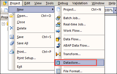
2. A screen for Create New Datastore will appear as below.
   1. Enter the datastore name (DS_BODS_HANA).
   2. Enter the datastore type as Database.
   3. Enter the database type as SAP HANA.
   4. Select the database version.
   5. Enter the SAP HANA database server name.
   6. Enter the port name for the SAP HANA database.
   7. Enter the user name and password.
   8. Tick “Enable automatic data transfer”.

Click on “Apply” and then the “OK” button.

The datastore “DS_BODS_HANA” will be displayed under the Datastore tab of the Local Object Library, as below.

3. Now we import a table into the datastore “DS_BODS_HANA”.
   1. Select the datastore “DS_BODS_HANA” and right-click.
   2. Select Import by Name.

4. A pop-up for Import by Name will appear as below.
   1. Select Type as Table.
   2. Enter the name as KNA1.
   3. Owner will be displayed as Hanauser.
   4. Click on the Import button.

The table will be imported into the “DS_BODS_HANA” datastore. To view the data in the table, follow the steps below.

1. Click on the table “KNA1” in the datastore “DS_BODS_HANA”.
2. Data will be displayed in tabular format.

Step 6) Define the project. A project groups and organizes related objects. A project can contain any number of jobs, workflows, and data flows.

1. Go to the Designer Project menu.
2. Select the New option.
3. Select the Project option.

A pop-up for new project creation appears as below. Enter the project name and click on the Create button. It will create a project folder, in our case BODS_DHK.

Step 7) Define the job. A job is a reusable object. It contains workflows and data flows. Jobs can be executed manually or on a schedule. To execute a BODS process, a job must be defined.

We create a job named JOB_Customer.

1. Select the project (BODS_DHK) created in the previous step, right-click, and select “New Batch Job”.
2. Rename it to “JOB_Customer”.

Step 8) Define the workflow.

1. Select the job “JOB_Customer” in the project area.
2. Click the workflow button on the tool palette. Click on the blank workspace area. A workflow icon will appear in the workspace.
3. Change the name of the workflow to “WF_Customer”.

Click the name of the workflow, and an empty view for the workflow appears in the workspace.

Step 9) Define the data flow.

1. Click on the workflow “WF_Customer”.
2. Click the data flow button on the tool palette. Click on the blank workspace area. A data flow icon will appear in the workspace.
3. Change the name of the data flow to “DF_Customer”.
4. The data flow also appears in the project area on the left, under the job name.

Step 10) Add objects to the data flow.

Inside the data flow, we provide instructions to transform source data into the desired form for the target table.

Three objects are used:

• An object for the source.
• An object for the target table.
• An object for the Query transform, which maps the columns from source to target.

Click on the data flow DF_Customer. A blank workspace will appear as below.

1. Specify the object for the source – Go to the datastore “ds_ecc”, select the table KNA1, and drag and drop it onto the blank data flow screen.
2. Specify the object for the target – Select the datastore “DS_BODS_HANA” from the repository and select the table KNA1.
3. Drag and drop it onto the workspace and select the “Make Target” option. There will now be two tables, one source and one target.

4. Query transformation – This is a tool used to retrieve data based on the input schema for a user specific condition, and to transport data from source to target.
   1. Select the Query Transform icon from the tool palette, and drag and drop it between the source and target objects in the workspace.
   2. Link the Query object to the source.
   3. Link the Query object to the target table.

Double-click on the Query icon to map columns from the input schema to the output schema. A mapping window appears, in which we do the following:

1. Source table KNA1 is selected.
2. Select all columns from the source table, right-click, and select Map to Output.
3. The target output is selected as Query, and the columns will be mapped.

Save and validate the project. Click on the Validate icon. A pop-up confirming validation success appears.

Step 11) Execute the job. To execute the job, follow the path below.

1. Select the project area icon to open the project, and select the created project.
2. Select the job and right-click.
3. Select the Execute option to execute the job.

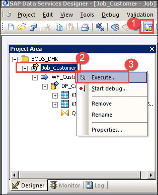
After executing the job, a Job Log window is displayed, in which all messages regarding the job appear. The last message will be “Job <job name> is completed successfully”.

Step 12) Validate and check the data in the SAP HANA database.

1. Log in to the SAP HANA database through SAP HANA Studio, and select the HANAUSER schema.
2. Select the KNA1 table in the Table node.
3. Right-click on the table KNA1 and select Open Data Preview.
4. The KNA1 data loaded by the BODS process will be displayed in the data preview screen.

A matching row count between the source table and this preview confirms the load completed correctly, and the job can then be scheduled from the Administrator for repeat runs.

FAQs