
dplyr in R Tutorial: Merge & Join Data with Examples
 Editorial Team
⚡ Smart Summary
dplyr merges and joins data frames in R with four verbs: left_join(), right_join(), inner_join() and full_join(). Its companion package tidyr then reshapes the joined result using gather(), spread(), separate() and unite().

Introduction to Data Analysis
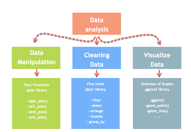
Before any join or reshaping verb makes sense, it helps to see where data manipulation fits. Data analysis can be divided into three parts:
- Extraction: First, we need to collect the data from many sources and combine them.
- Transform: This step involves the data manipulation. Once we have consolidated all the sources of data, we can begin to clean the data.
- Visualize: The last move is to visualize our data to check irregularity.
The diagram below shows how the three stages connect.
One of the most significant challenges faced by data scientists is data manipulation. Data is never available in the desired format. Data scientists need to spend at least half of their time cleaning and manipulating the data. That is one of the most critical assignments in the job. If the data manipulation process is not complete, precise and rigorous, the model will not perform correctly.
R dplyr
R has a package called dplyr that handles data transformation. It is built around a small set of core verbs — filter(), select(), arrange(), mutate() and summarise() — plus a family of join functions. Once the data is in shape, ggplot2 can visualize it.
We will learn how to use the dplyr package to manipulate a Data Frame. If R is not installed yet, follow the R and RStudio setup steps, then run install.packages(“dplyr”).
Merge Data with dplyr
dplyr provides a nice and convenient way to combine datasets. We may have many sources of input data, and at some point, we need to combine them. A join with dplyr adds variables to the right of the original dataset.
dplyr Joins
Following are four important types of joins used in dplyr to merge two datasets. All four take the same arguments — the two tables and the key — and differ only in which unmatched rows survive:
| Function | Objective | Arguments | Multiple keys |
|---|---|---|---|
| left_join() | Merge two datasets. Keep all observations from the origin table | x, y, by = “ID” | x, y, by = c(“ID”, “ID2”) |
| right_join() | Merge two datasets. Keep all observations from the destination table | x, y, by = “ID” | x, y, by = c(“ID”, “ID2”) |
| inner_join() | Merge two datasets. Exclude all unmatched rows | x, y, by = “ID” | x, y, by = c(“ID”, “ID2”) |
| full_join() | Merge two datasets. Keep all observations | x, y, by = “ID” | x, y, by = c(“ID”, “ID2”) |
These four verbs map onto the LEFT, RIGHT, INNER and FULL OUTER joins of SQL. Base R reaches the same results through the all, all.x and all.y arguments of merge().
We will study all the join types via an easy example.
First of all, we build two datasets. Table 1 contains two variables, ID and y, whereas Table 2 gathers ID and z. In each situation, we need to have a key-pair variable. In our case, ID is our key variable. The function will look for identical values in both tables and bind the returning values to the right of table 1. The figure below shows the two tables side by side.

library(dplyr)
df_primary <- tribble(
  ~ID, ~y,
   "A", 5,
   "B", 5,
   "C", 8,
   "D", 0,
  "F", 9)
df_secondary <- tribble(
  ~ID, ~z,
   "A", 30,
   "B", 21,
   "C", 22,
   "D", 25,
   "E", 29)
dplyr left_join()
The most common way to merge two datasets is to use the left_join() function. The picture below shows that the key-pair matches rows A, B, C and D, while E and F are left over. With left_join(), we keep all the rows in the original table and ignore the rows that have no key-pair in the destination table. In our example, the value E does not exist in table 1, so that row is dropped. The value F comes from the origin table, so it is kept after the left_join() and returns NA in the column z.
Example of dplyr left_join()
The diagram below reproduces what happens during a left_join().

left_join(df_primary, df_secondary, by ='ID')
Output:
##
# A tibble: 5 x 3
##      ID   y.x   y.y
##   <chr> <dbl> <dbl>
## 1     A     5    30
## 2     B     5    21
## 3     C     8    22
## 4     D     0    25
## 5     F     9    NA
Note that when both tables carry a column of the same name, dplyr disambiguates them with the .x and .y suffixes shown above.
dplyr right_join()
The right_join() function works exactly like left_join(). The only difference is the row dropped. The value E, available in the destination data frame, exists in the new table and takes the value NA for the column y.
Example of dplyr right_join()
The diagram below shows the mirror image.

right_join(df_primary, df_secondary, by = 'ID')
Output:
##
# A tibble: 5 x 3
##      ID   y.x   y.y
##   <chr> <dbl> <dbl>
## 1     A     5    30
## 2     B     5    21
## 3     C     8    22
## 4     D     0    25
## 5     E    NA    29
dplyr inner_join()
When unmatched observations are of no use at all, we can return only the rows that exist in both datasets. This is the right choice when we need a complete dataset and do not want to impute missing values with the mean or median.
The inner_join() function comes to help here. It excludes the unmatched rows on both sides.
Example of dplyr inner_join()
The diagram below highlights the four IDs that survive the join.

inner_join(df_primary, df_secondary, by ='ID')
Output:
##
# A tibble: 4 x 3
##      ID   y.x   y.y
##   <chr> <dbl> <dbl>
## 1     A     5    30
## 2     B     5    21
## 3     C     8    22
## 4     D     0    25
dplyr full_join()
Finally, the full_join() function keeps all observations and replaces missing values with NA.
Example of dplyr full_join()
The diagram below shows every ID from both tables surviving the join.

full_join(df_primary, df_secondary, by = 'ID')
Output:
## # A tibble: 6 x 3
##      ID   y.x   y.y
##   <chr> <dbl> <dbl>
## 1     A     5    30
## 2     B     5    21
## 3     C     8    22
## 4     D     0    25
## 5     F     9    NA
## 6     E    NA    29
Multiple Key pairs
Last but not least, we can have multiple keys in our dataset. Consider the following dataset where we have years and a list of products bought by the customer. The screenshot below shows the two tables and the ID and year columns that together identify a row.
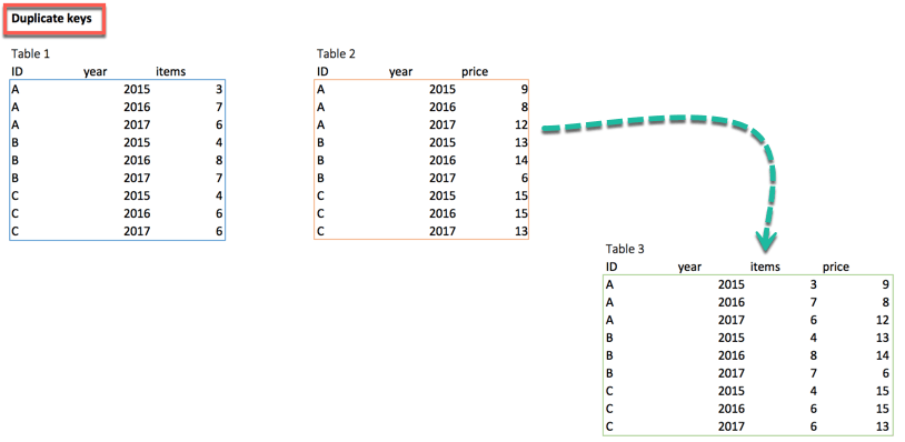
If we join both tables on ID alone, every year is matched against every year and the row count explodes. To remedy the situation, we can pass two key-pair variables. That is, ID and year, which appear in both datasets. We can use the following code to merge table 1 and table 2:
df_primary <- tribble(
  ~ID, ~year, ~items,
  "A", 2015,3,
  "A", 2016,7,
  "A", 2017,6,
  "B", 2015,4,
  "B", 2016,8,
  "B", 2017,7,
  "C", 2015,4,
  "C", 2016,6,
  "C", 2017,6)
df_secondary <- tribble(
  ~ID, ~year, ~prices,
  "A", 2015,9,
  "A", 2016,8,
  "A", 2017,12,
  "B", 2015,13,
  "B", 2016,14,
  "B", 2017,6,
  "C", 2015,15,
  "C", 2016,15,
  "C", 2017,13)
left_join(df_primary, df_secondary, by = c('ID', 'year'))
Output:
## # A tibble: 9 x 4
##      ID  year items prices
##   <chr> <dbl> <dbl>  <dbl>
## 1     A  2015     3      9
## 2     A  2016     7      8
## 3     A  2017     6     12
## 4     B  2015     4     13
## 5     B  2016     8     14
## 6     B  2017     7      6
## 7     C  2015     4     15
## 8     C  2016     6     15
## 9     C  2017     6     13
Since dplyr 1.1.0 (January 2023) the same key can be written as join_by(ID, year), and dplyr now warns about unexpected many-to-many matches, as the dplyr 1.1.0 joins announcement explains.
Data Cleaning Functions in R
Merging solves only half of the problem, because the combined table still has to be reshaped. Following are the four important functions to tidy (clean) the data:
| Function | Objective | Arguments |
|---|---|---|
| gather() | Transform the data from wide to long | (data, key, value, na.rm = FALSE) |
| spread() | Transform the data from long to wide | (data, key, value) |
| separate() | Split one variable into two | (data, col, into, sep = “”, remove = TRUE) |
| unite() | Unite two variables into one | (data, col, conc, sep = “”, remove = TRUE) |
Version note: gather() and spread() were superseded by pivot_longer() and pivot_wider() in tidyr 1.0.0, and separate() by the separate_wider_delim() family in tidyr 1.3.0. Superseded functions still run, so every example below works, but new code should prefer the newer families shown in the tidyr pivoting vignette. unite() remains current.
We use the tidyr package, part of the tidyverse collection for manipulating, cleaning and visualizing data. If R was installed with Anaconda, the package is already available from https://anaconda.org/r/r-tidyr.
If not installed already, enter the following command to install tidyr:
install.packages("tidyr")
gather()
The objective of the gather() function is to transform the data from wide to long.
Syntax
gather(data, key, value, na.rm = FALSE)
Arguments:
-data: The data frame used to reshape the dataset
-key: Name of the new column created
-value: Select the columns used to fill the key column
-na.rm: Remove missing values. FALSE by default
Example
Below, we can visualize the concept of reshaping wide to long. We want to create a single column named growth, filled by the rows of the quarter variables. The figure below shows the wide table on the left and the reshaped long table on the right.

library(tidyr)
# Create a messy dataset
messy <- data.frame(
  country = c("A", "B", "C"),
  q1_2017 = c(0.03, 0.05, 0.01),
  q2_2017 = c(0.05, 0.07, 0.02),
  q3_2017 = c(0.04, 0.05, 0.01),
  q4_2017 = c(0.03, 0.02, 0.04))
messy
Output:
##   country q1_2017 q2_2017 q3_2017 q4_2017
## 1       A    0.03    0.05    0.04    0.03
## 2       B    0.05    0.07    0.05    0.02
## 3       C    0.01    0.02    0.01    0.04
# Reshape the data
tidier <-messy %>%
gather(quarter, growth, q1_2017:q4_2017)
tidier
Output:
##    country quarter growth
## 1        A q1_2017   0.03
## 2        B q1_2017   0.05
## 3        C q1_2017   0.01
## 4        A q2_2017   0.05
## 5        B q2_2017   0.07
## 6        C q2_2017   0.02
## 7        A q3_2017   0.04
## 8        B q3_2017   0.05
## 9        C q3_2017   0.01
## 10       A q4_2017   0.03
## 11       B q4_2017   0.02
## 12       C q4_2017   0.04
In the gather() function, we create two new variables, quarter and growth, because our original dataset has one group variable, country, and the key-value pairs. In tidyr 1.0.0 and later the same reshape is written as pivot_longer(messy, cols = q1_2017:q4_2017, names_to = “quarter”, values_to = “growth”).
spread()
The spread() function does the opposite of gather().
Syntax
spread(data, key, value)
arguments:
data: The data frame used to reshape the dataset
key: Column to reshape long to wide
value: Rows used to fill the new column
Example
We can reshape the tidier dataset back to messy with spread().
# Reshape the data
messy_1 <- tidier %>%
  spread(quarter, growth)
messy_1
Output:
##   country q1_2017 q2_2017 q3_2017 q4_2017
## 1       A    0.03    0.05    0.04    0.03
## 2       B    0.05    0.07    0.05    0.02
## 3       C    0.01    0.02    0.01    0.04
The modern equivalent is pivot_wider(tidier, names_from = quarter, values_from = growth).
separate()
The separate() function splits a column into two according to a separator. This function is helpful in situations where the variable is a date. Our analysis can require focusing on month and year, and we want to separate the column into two new variables.
Syntax
separate(data, col, into, sep= "", remove = TRUE)
arguments:
-data: The data frame used to reshape the dataset
-col: The column to split
-into: The name of the new variables
-sep: Indicates the symbol used that separates the variable, i.e.:  "-", "_", "&"
-remove: Remove the old column. By default sets to TRUE.
Example
We can split the quarter from the year in the tidier dataset by applying the separate() function.
separate_tidier <-tidier %>%
separate(quarter, c("Qrt", "year"), sep ="_")
head(separate_tidier)
Output:
##   country Qrt year growth
## 1       A  q1 2017   0.03
## 2       B  q1 2017   0.05
## 3       C  q1 2017   0.01
## 4       A  q2 2017   0.05
## 5       B  q2 2017   0.07
## 6       C  q2 2017   0.02
unite()
The unite() function concatenates two columns into one.
Syntax
unite(data, col, conc ,sep= "", remove = TRUE)
arguments:
-data: The data frame used to reshape the dataset
-col: Name of the new column
-conc: Name of the columns to concatenate
-sep: Indicates the symbol used that unites the variable, i.e:  "-", "_", "&"
-remove: Remove the old columns. By default, sets to TRUE
Example
In the above example, we separated quarter from year. What if we want to merge them? We use the following code:
unit_tidier <- separate_tidier %>%
  unite(Quarter, Qrt, year, sep ="_")
head(unit_tidier)
Output:
##   country Quarter growth
## 1       A q1_2017   0.03
## 2       B q1_2017   0.05
## 3       C q1_2017   0.01
## 4       A q2_2017   0.05
## 5       B q2_2017   0.07
## 6       C q2_2017   0.02
The reshaped data frame is now ready for the modelling steps covered in the rest of the R tutorial series.
