Adjacency List and Matrix Representation of Graph

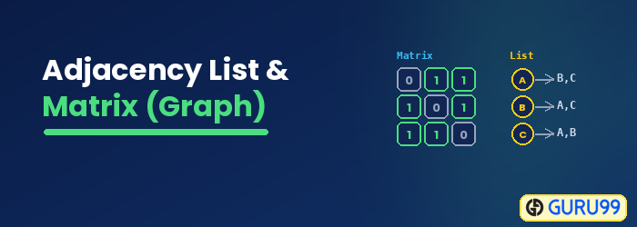
Even though they look different, all types of graphs can be represented in a similar way. There are generally two types of graph representation:

1. Adjacency Matrix
2. Adjacency List

Adjacency List

An adjacency list consists of linked lists. Each vertex is considered an array index, and each element represents a linked list. These linked lists contain the vertices that share an edge with the index vertex.

Here is an example of an adjacency list:

Let a graph contain V number of vertices and E number of edges. The space complexity of the adjacency list is O(V + E), which scales with the number of real edges rather than every possible pair of vertices.

Worst-case space complexity becomes O(V²) if the given graph is a complete graph, since every vertex then connects to every other vertex.

Adjacency Matrix

An adjacency matrix is composed of a 2D array. For a graph with V vertices, the size of the matrix will be V × V.

Say matrix[i][j] = 5. It means there is an edge between node i and node j where the weight is 5.

Let us look at the following graph and its adjacency matrix:

We built the 2D array using these steps:

Step 1) Vertex A has a direct edge with B, and the weight is 5. So, the cell in row A and column B will be filled with 5. The rest of the cells in row A will be filled with zero.

Step 2) Vertex B has a direct edge with C, and the weight is 4. So, the cell in row B and column C will be filled with 4. The remaining cells in row B will be filled with zero, since B has no outgoing edge to any other node.

Step 3) Vertex C has no direct edges with any other vertices. So, row C will be filled with zeros.

Step 4) Vertex D has a directed edge with A and C.

• The cell in row D and column A will have a value of 7. The cell in row D and column C will have a value of 2.
• The rest of the cells in row D will be filled with zeros.

Step 5) Vertex E has a directed edge with B and D. The cell in row E and column B will have a value of 6. The cell in row E and column D will have a value of 3. The rest of the cells in row E will be filled with zeros.

Here are some points to notice:

• The graph has no self-loops when the primary diagonal of the adjacency matrix is 0.
• The graph is a directed graph if the cells at (a, b) and (b, a) do not hold the same value. Otherwise, the graph is undirected.
• The graph is a weighted graph if the value of any cell is greater than 1.

The main problem with the adjacency matrix is that it requires squared space. Even edges that do not exist still allocate cells in memory.

For example, if we have a graph with 100 nodes, then 10,000 cells are needed to store it in RAM. With fewer edges in the graph, allocating such large memory can be wasteful. So the space complexity using the adjacency matrix is O(N²), where N is the number of nodes in the graph.

Adjacency List vs Adjacency Matrix

Before choosing a representation, it helps to compare both models side by side across the operations that dominate real graph workloads:

Operation	Adjacency Matrix	Adjacency List
Space complexity	O(V²)	O(V + E)
Add a vertex	O(V²)	O(1)
Add an edge	O(1)	O(1)
Remove an edge	O(1)	O(E)
Check if edge (i, j) exists	O(1)	O(degree of i)
Iterate over neighbours of i	O(V)	O(degree of i)
Best for	Dense graphs, frequent edge queries	Sparse graphs, traversal-heavy tasks

In short, adjacency matrix wins on constant-time edge lookups, while adjacency list wins on memory and neighbour iteration, which is why algorithms such as BFS, DFS, and Dijkstra usually pair with adjacency lists.

Advantages and Disadvantages of Graph Representation

Each representation carries its own trade-offs. Knowing the strengths and weaknesses of both models helps you pick the right one for the problem you are solving.

Advantages of Adjacency Matrix:

• Constant-time O(1) edge-existence queries between any pair of vertices.
• Fixed indexing makes matrix-based algorithms such as Floyd-Warshall and transitive closure easy to implement.
• Weighted edges fit naturally in a single matrix cell.

Disadvantages of Adjacency Matrix:

• Wastes O(V²) memory when the graph is sparse.
• Adding a new vertex requires resizing the entire matrix.
• Iterating over neighbours of a single vertex takes O(V) even when the vertex has only a few edges.

Advantages of Adjacency List:

• Uses only O(V + E) memory, which is close to the real edge count in sparse graphs.
• Adding a new vertex or edge is O(1).
• Traversal algorithms such as BFS and DFS iterate neighbours in O(degree), giving overall O(V + E) running time.

Disadvantages of Adjacency List:

• Checking whether a specific edge exists takes O(degree) time instead of O(1).
• Cache locality is weaker because linked lists are scattered across memory.
• Weighted edges need a companion field or a list of pairs, slightly complicating the data structure.

When to Use Adjacency List vs Adjacency Matrix

The choice of representation depends on the density of the graph and the operations you run most often. Use this quick guide to pick the right structure:

• Prefer the adjacency matrix when the graph is dense (E is close to V²), when edges rarely change, and when your algorithm asks “is there an edge between i and j?” many times.
• Prefer the adjacency list when the graph is sparse (E is much smaller than V²), when the vertex or edge set grows during execution, and when you traverse the graph with BFS, DFS, or Dijkstra’s shortest-path algorithm.
• Prefer a mixed model (adjacency list plus a hash set of edges) when you need both fast neighbour iteration and O(1) edge queries, at the cost of extra memory.

Modern graph libraries such as NetworkX and igraph default to adjacency lists because most real-world graphs — social networks, road maps, web pages, package dependencies — are sparse and traversal-heavy.

FAQs